Fig. 1. (a) Configuration of a unit block. P, period; wx, width; wy, length; h, height; α, orientation angle. (b) Configurations of Au block to accomplish complex modulation. The color bars are amplitude range of [0, 0.5] and phase range of [−π,π], which are the same as in (c) and (d). (c), (d) Amplitude and phase conversion over 500–1500 nm range for the 10 configurations specified in the red rectangle in (b). (e) Experimental setup. PBS, polarization beam splitter; LCP, LCP generator, consisting of a polarizer and a λ/4 wave plate; RCP, RCP filter, composed of a polarizer and a λ/4 wave plate.

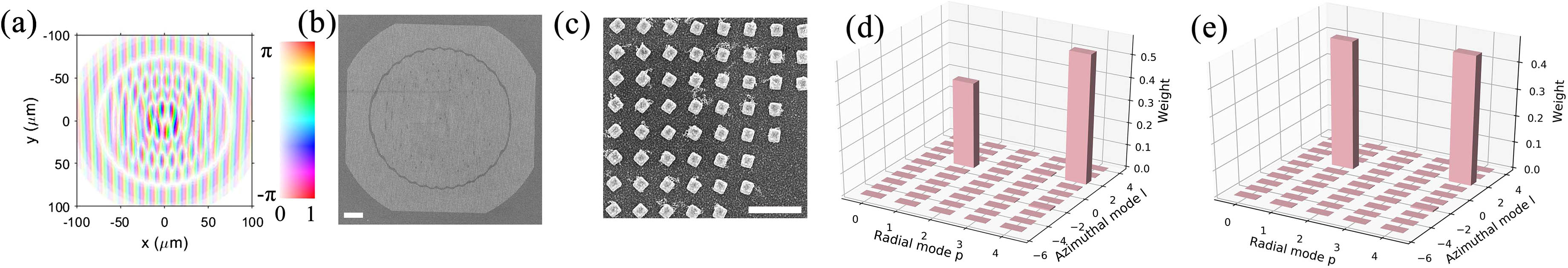
Fig. 2. (a) Rounded complex pattern to convert the fundamental Gaussian beam into a combination of LG42 and LG11 directed to g→1=(1,0), with angles θ=5° and θ=10°. The assigned weight has a ratio of LG42∶LG11=6∶4. (b) Overall scanning electron microscope (SEM) image. (c) Zoomed SEM image. (d) LG decomposition results for the complex pattern in (a) without deflection. (e) LG decomposition results for the modes combination of LG42∶LG11=1∶1. Scale bar: 20 μm in (b); 1 μm in (c).

Fig. 3. Gaussian distribution under three scenarios: “pessimistic,” “neutral,” “optimistic.”

Fig. 4. Error distribution for four different configurations with 10 nm deviation along the width and length of the Au block. The first and third columns are the absolute error over different width and length. The second and fourth columns are the Gaussian-distributed error from the desired configuration. For the four configurations we selected here, the width wx is fixed at 200 nm. The lengths wy are (a) 220 nm, (b) 225 nm, (c) 230 nm, and (d) 250 nm.

Fig. 5. Experimental results: broadband performance of meta-converters. (a)–(d) Diffraction patterns with metasurface designed for LG42∶LG11=6∶4. The test wavelength and the measurement distance from the metasurface are all labeled with the beam profile. First row: simulation. Second row: experiments. (e) Simulated broadband performance for the meta-converter of LG42∶LG11=6∶4 in terms of error and efficiency. (f) Metasurface contains modes of LG11∶LG22∶LG23=3∶4∶5. The left edge corresponds to zero deflection for all figures. Scale bar for all: 200 μm.

Fig. 6. (a) Amplitude conversion and (b) phase conversion under different wy and orientation angle α when x is set at 200 nm and incident source is set at 1000 nm.

Fig. 7. First column: amplitude pattern. Second column: phase pattern. Third column: LG decomposition results. (a) Rounded complex pattern, featuring LG42∶LG11=1∶1. (b) Complex pattern with a Gaussian noise N(0,0.052) applied to the amplitude. (c) Complex pattern with a Gaussian noise N(0.05,0.052) applied to the amplitude.

Table 1. Three Scenarios of Gaussian Distribution

Table 2. Parameters Approximation^a