Mie Theory Simulation and Empirical Analysis of Mass-Specific Backscattering Properties of Suspended Particles in the Yellow and East China Seas

Shuang Cao; Bing Han; Jianhua Zhu; Zhifeng Li

doi:10.3788/LOP202259.1301002

Journals >Laser & Optoelectronics Progress >Volume 59 >Issue 13 >Page 1301002 > Article

Laser & Optoelectronics Progress
Vol. 59, Issue 13, 1301002 (2022)

Mie Theory Simulation and Empirical Analysis of Mass-Specific Backscattering Properties of Suspended Particles in the Yellow and East China Seas

Shuang Cao, Bing Han^*, Jianhua Zhu, and Zhifeng Li

Author Affiliations

National Ocean Technology Center, Tianjin 300111, China

show less

DOI: 10.3788/LOP202259.1301002 Cite this Article Set citation alerts

Shuang Cao, Bing Han, Jianhua Zhu, Zhifeng Li. Mie Theory Simulation and Empirical Analysis of Mass-Specific Backscattering Properties of Suspended Particles in the Yellow and East China Seas[J]. Laser & Optoelectronics Progress, 2022, 59(13): 1301002 Copy Citation Text

show less

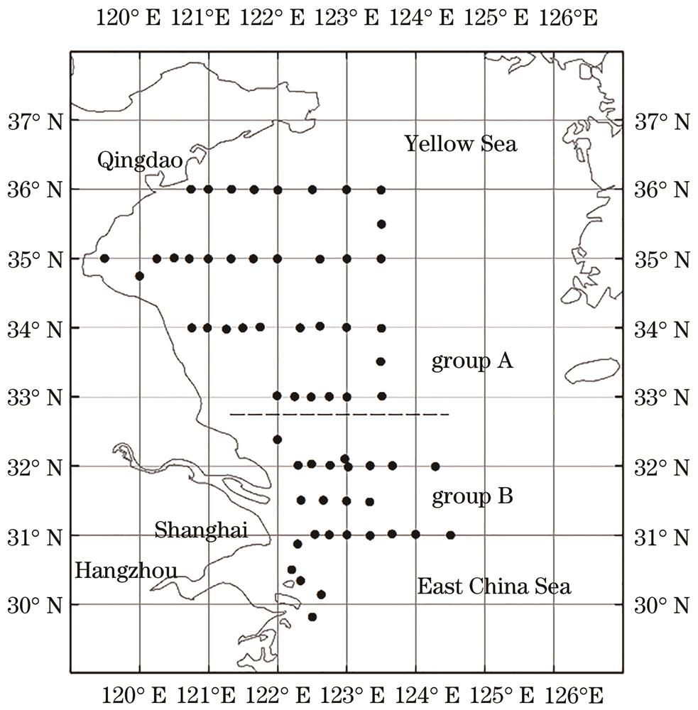
Fig. 1. Diagram of observation station during the autumn cruise carried out in 2003 over the Yellow and East China Seas

Download full size

bbp* spectra for all of the data measured during the cruise, and the average spectrum shown with one standard deviation range (x¯±s)

Fig. 2.

b_{b p}^{*}

spectra for all of the data measured during the cruise, and the average spectrum shown with one standard deviation range (

\bar{x}

±s)

Download full size

Fig. 3. Variations of backscattering efficiency

Q_{b b}

of spherical homogeneous particles with particle diameter D for various wavelengths

Download full size

$Variations of backscattering efficiency Qbb with particle diameter D for various real part of relative refractive index n and imaginary part of relative refractive index n′. (a) Real part of relative refractive index n; (b) imaginary part of relative refractive index n′$

Fig. 4. Variations of backscattering efficiency

Q_{b b}

with particle diameter D for various real part of relative refractive index n and imaginary part of relative refractive index n′. (a) Real part of relative refractive index n; (b) imaginary part of relative refractive index n′

Download full size

Fig. 5. Theoretical relationship between

b_{b p}^{*} (532)

and ξ. In this figure, the light dashed lines represent the algae particles, the light solid lines represent the inorganic mineral particles, and the two black dotted lines represent the fitting curves of algae particles and inorganic mineral particles under the average condition

Download full size

$Theoretical relationship between bbp*(532) and the real part of the relative refractive index n of particles for various apparent density ρa when ξ is 4.0. The scattered points marked in the figure represent the bbp*(532) theoretical values of different algae and inorganic mineral particles at their corresponding n and ρa$

Fig. 6. Theoretical relationship between

b_{b p}^{*} (532)

and the real part of the relative refractive index n of particles for various apparent density ρ_a when ξ is 4.0. The scattered points marked in the figure represent the

b_{b p}^{*} (532)

theoretical values of different algae and inorganic mineral particles at their corresponding n and ρ_a

Download full size

Fig. 7.

b_{b p}^{*}

spectra of Dunaliella bioculata simulated under different n′ value

Download full size

Fig. 8. Relationship between

b_{b p}^{*}

spectral slope η and characteristic parameters of particles. (a) η versus suspended particle concentration C_SPM; (b) η versus the proportion of organic particles mass concentration C_POM/C_SPM

Download full size

Fig. 9. Relationship between

b_{b p} (532)

and C_SPM in the logarithmic coordinate system

Download full size

Fig. 10. Relational model between the measured

b_{b p}^{*} (532)

and C_POM/C_SPM. The dashed line and thin solid line in the figure represent the simulation results with different values of particle size distribution slopes ξ, the circular scatter points represent in situ sampling points, and the bold solid line represents the power-law fitting results for in situ data

Download full size

Fig. 11. Relational model between the measured

b_{b p}^{*} (532)

and C_POM/C_SPMfor the group A and group B. (a) Group A; (b) group B

Download full size

Parameter	Minimum	Maximum	Average	Median	SD	CV /%
$b_{b p} (442)$ /（10^-2 m^-1）	0.38	111.24	8.49	0.96	19.00	223.0
$b_{b p} (488)$ /（10^-2 m^-1）	0.27	89.14	7.20	0.84	16.00	216.0
$b_{b p} (532)$ /（10^-2 m^-1）	0.19	88.66	7.02	0.70	15.00	220.0
$b_{b p} (589)$ /（10^-2 m^-1）	0.15	87.70	6.76	0.60	15.00	225.0
$b_{b p} (676)$ /（10^-2 m^-1）	0.11	75.57	5.84	0.51	13.00	225.0
$b_{b p} (852)$ /（10^-2 m^-1）	0.07	63.38	4.85	0.42	11.00	226.0
C_SPM /（g·m^-3）	0.40	95.30	8.91	1.90	18.00	197.0
C_PIM /（g·m^-3）	0.10	88.60	7.66	1.00	17.00	216.0
C_POM /（g·m^-3）	0.20	6.70	1.26	1.00	1.08	86.3
C_POM/C_SPM/10^-1	0.48	8.42	4.44	4.55	2.46	55.5
$b_{b p}^{*}$ spectral slop η	0.53	2.46	1.29	1.22	0.48	37.4
$b_{b p}^{*} (532)$ /（10^-3 m²·g^-1）	2.22	17.50	5.43	4.58	2.89	53.3
$b_{b p}^{*} (676)$ /（10^-3 m²·g^-1）	1.53	14.11	4.12	3.21	2.55	61.8

Table 1. Statistical results of in situ measured data

Parameter	Value（Increments are given in parentheses）	Reference
λ /nm	442，488，532，589，676，852	—
D /μm	0.02（Set 200 points at logarithmic intervals）200	Babin et al.^［16］；Zhou et al.^［22］
n	1.01（0.02）1.27	Mobley^［19］；Bricaud et al.^［23］
n′	0，0.001，0.005	Bricaud et al.^［18］；Ahn et al.^［24］
ξ	3.0（0.2）5.0	Babin et al.^［16］
ρ_a /（10⁶ g·m^-3）	0.3（0.3）5.1	Woźniak et al.^［17］；Aas^［25］

Table 2. Setting of main parameters of Mie calculations

Algae particle type	n	ρ_a/（10⁶ g·m^-3）	$b_{b p}^{*} (532)$ /（10^-3 m²·g^-1）
Algae particle type	n	ρ_a/（10⁶ g·m^-3）	ξ=3.8	ξ=4.0	ξ=4.2
Average	1.0587	0.535	1.95	4.09	8.39
Green algae	1.0558	0.492	1.88	3.96	8.14
Diatoms	1.0566	0.614	1.55	3.27	6.72
Blue-green algae	1.0574	0.501	1.96	4.13	8.48
Dinoflagellates	1.0604	0.496	2.22	4.66	9.53
Coccolithophorids	1.0631	0.570	2.12	4.44	9.08

Table 3.

b_{b p}^{*} (532)

values of different algal particles, assuming n′=0 and ξ value as indicated

Mineral particle type	n	ρ_a/（10⁶ g·m^-3）	$b_{b p}^{*} (532)$ /（10^-3 m²·g^-1）
Mineral particle type	n	ρ_a/（10⁶ g·m^-3）	ξ=3.8	ξ=4.0	ξ=4.2
Average	1.168	2.61	4.68	9.12	17.35
Opal	1.075	1.90	0.94	1.95	3.93
Quartz	1.156	2.65	3.83	7.41	14.08
Kaolinite	1.164	2.65	4.30	8.30	15.73
Montmorillonite	1.167	2.50	4.72	9.13	17.32
Calcite	1.173	2.71	4.69	9.10	17.24
Gibbsite	1.177	2.42	5.49	10.67	20.25
Illite	1.179	2.80	4.87	9.46	17.94
Chlorite	1.206	3.00	6.09	11.93	22.65
Aragonite	1.218	2.83	7.18	14.16	27.00

Table 4.

b_{b p}^{*} (532)

of the typical mineral particles in coastal waters, assuming n′=0 and ξ value as indicated

Mineral particle type	Illite	Chlorite	Kaolinite	Montmorillonite	Reference
Proportion /%	61.00	17.06	13.94	8.00	Wei et al.^［30］
	61.80	9.40	13.00	15.80	Song et al.^［31］
	61.90	10.00	13.10	15.00	Zhang et al.^［32］
Average /%	62.00	12.00	13.00	13.00	This study

Table 5. Type and content ratio of main inorganic minerals in the Yellow and East China Seas

ξ	$b_{b p}^{*} (532)$ /（10^-3 m²·g^-1）（Changing rate/%）
ξ	n′=0.001	n′=0.005
3.6	0.64（-15.76）	0.55（-28.11）
3.8	1.43（-7.79）	1.31（-15.38）
4.0	3.15（-3.63）	3.01（-7.99）
4.2	6.60（-1.72）	6.44（-4.18）
4.4	13.03（-0.88）	12.84（-2.27）

Table 6.

b_{b p}^{*} (532)

value at different imaginary parts of relative refractive index n′ and its changing rate compared with the case without absorption, taking Diatoms as example

Parameter	C_SPM	C_PIM	C_POM	C_POM/C_SPM	$b_{b p} (532)$	$b_{b p}^{*} (532)$	η
C_SPM	1.00
C_PIM	1.00	1.00
C_POM	0.93	0.92	1.00
C_POM/C_SPM	-0.62	-0.62	-0.58	1.00
$b_{b p} (532)$	0.96	0.96	0.87	-0.61	1.00
$b_{b p}^{*} (532)$	0.43	0.43	0.37	-0.62	0.58	1.00
η	-0.51	-0.50	-0.61	0.75	-0.48	-0.54	1.00