• Photonics Research
  • Vol. 6, Issue 10, 929 (2018)
Ernesto Jimenez-Villar1、2、*, M. C. S. Xavier2、3, Niklaus U. Wetter1, Valdeci Mestre4, Weliton S. Martins5, Gabriel F. Basso6, V. A. Ermakov7, F. C. Marques7, and Gilberto F. de Sá8
Author Affiliations
  • 1Instituto de Pesquisas Energéticas e Nucleares, CNEN_IPEN, São Paulo, SP 05508-000, Brazil
  • 2Departamento de Física, Universidade Federal da Paraíba, João Pessoa, PB 58051-970, Brazil
  • 3Departamento de Física, Universidade Estadual da Paraíba, Araruna, PB 58233-000, Brazil
  • 4CCEA, Universidade Estadual da Paraíba, Patos, PB 58706-560, Brazil
  • 5Departamento de Física, Universidade Federal Rural de Pernambuco, Recife, PE 52171-900, Brazil
  • 6Departamento de Informática, Universidade Federal da Paraíba, Joao Pessoa, PB 58055-000, Brazil
  • 7Departamento de Física Aplicada, Universidade Estadual de Campinas, Campinas, SP 13083-859, Brazil
  • 8Química Fundamental, Universidade Federal de Pernambuco, Recife, PE 50670-901, Brazil
  • show less
    DOI: 10.1364/PRJ.6.000929 Cite this Article Set citation alerts
    Ernesto Jimenez-Villar, M. C. S. Xavier, Niklaus U. Wetter, Valdeci Mestre, Weliton S. Martins, Gabriel F. Basso, V. A. Ermakov, F. C. Marques, Gilberto F. de Sá. Anomalous transport of light at the phase transition to localization: strong dependence with incident angle[J]. Photonics Research, 2018, 6(10): 929 Copy Citation Text show less
    For sample [140×1010 NPs·mL−1], transmitted total intensity versus incidence angle. (a) Transmission coefficient for incidence angles θ of 0°, 30°, 60°, and 70° as a function of slab thickness (d). The black, red, blue, and green dotted lines represent the fitting β(d0+d)−2 with experimental points for 0°, 30°, 60°, and 70°, respectively. (b) Relative conductance G(d;θ) as a function of d; (c) asymptotic values of relative conductance G(∞;θ) as a function of the incidence angle.
    Fig. 1. For sample [140×1010  NPs·mL1], transmitted total intensity versus incidence angle. (a) Transmission coefficient for incidence angles θ of 0°, 30°, 60°, and 70° as a function of slab thickness (d). The black, red, blue, and green dotted lines represent the fitting β(d0+d)2 with experimental points for 0°, 30°, 60°, and 70°, respectively. (b) Relative conductance G(d;θ) as a function of d; (c) asymptotic values of relative conductance G(;θ) as a function of the incidence angle.
    Measurement of intensity profiles at the sample output face. (a) For 140×1010 NPs·mL−1 (localization) and 14×1010 NPs·mL−1 (diffusive regime), G(∞;θ)=I(0°)/I(θ) versus incidence angle. (b) For 140×1010 NPs·mL−1, (left, red) ωeff and (right, black) the relative effective width (normalized width) versus incidence angle; (c) for 14×1010 NPs·mL−1 (diffusive), (left, red) ωeff and (right, black) the relative effective width (normalized width) are also plotted as a function of the incidence angle. The error bars are the statistic standard deviation of relative intensity and effective width (ωeff). For 140×1010 NPs·mL−1 (localization), normalized intensity profiles for incidence angles of (d) 0°, (e) 30°, (f) 60°, and (g) 70°. Red arrows point quicker decay for large r. The intensity profiles are fitted to exp(−2(|r|/σ))1+ν (red solid lines), where 0<ν<1.
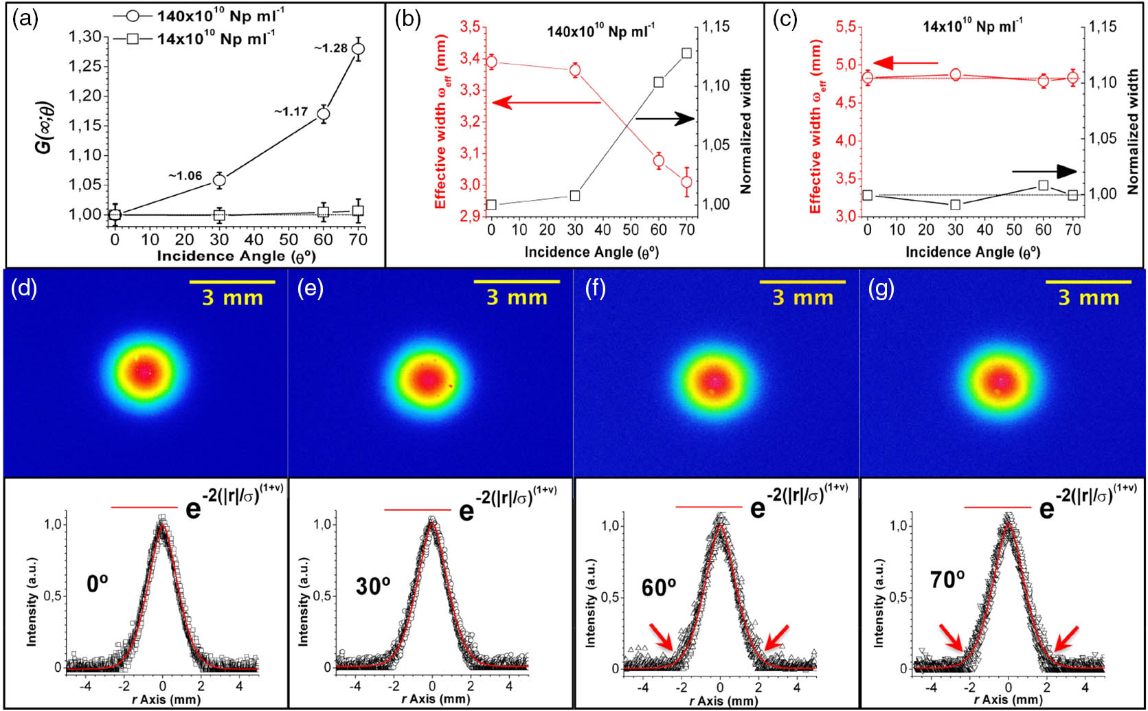
    Fig. 2. Measurement of intensity profiles at the sample output face. (a) For 140×1010  NPs·mL1 (localization) and 14×1010  NPs·mL1 (diffusive regime), G(;θ)=I(0°)/I(θ) versus incidence angle. (b) For 140×1010  NPs·mL1, (left, red) ωeff and (right, black) the relative effective width (normalized width) versus incidence angle; (c) for 14×1010  NPs·mL1 (diffusive), (left, red) ωeff and (right, black) the relative effective width (normalized width) are also plotted as a function of the incidence angle. The error bars are the statistic standard deviation of relative intensity and effective width (ωeff). For 140×1010  NPs·mL1 (localization), normalized intensity profiles for incidence angles of (d) 0°, (e) 30°, (f) 60°, and (g) 70°. Red arrows point quicker decay for large r. The intensity profiles are fitted to exp(2(|r|/σ))1+ν (red solid lines), where 0<ν<1.
    For 140×1010 NPs·mL−1 (localization regime), coherent backscattering cones for incidence angles of (a) 0°, (b) 30°, (c) 60°, and (d) 70°. The red solid lines represent the background intensity (incoherently backscattered photons), taking into account the internal reflection at the interface of silica–air (light coming out of the cuvette). The coherent backscattering cones obtained by subtraction of the background intensity are shown below each graph. (e) (Left, red) ICBC and (right, black) IR (%) as a function of the incidence angle; (f) (left, red) half-width of backscattering cone and (right, black) lT0 as a function of IR (%); (g) (left, red) asymptotic values of relative conductance (G(∞;θ)), extracted from the transmission and propagation experiments, and (right, black) enhancement factor of backscattering cone as a function of IR (%). The black dotted lines in (f) and (g) represent linear fittings with the experimental points. Error bars correspond to the standard deviation of the intensity of the backscattering cone (ICBC) and the calculated IR (%).
    Fig. 3. For 140×1010  NPs·mL1 (localization regime), coherent backscattering cones for incidence angles of (a) 0°, (b) 30°, (c) 60°, and (d) 70°. The red solid lines represent the background intensity (incoherently backscattered photons), taking into account the internal reflection at the interface of silica–air (light coming out of the cuvette). The coherent backscattering cones obtained by subtraction of the background intensity are shown below each graph. (e) (Left, red) ICBC and (right, black) IR (%) as a function of the incidence angle; (f) (left, red) half-width of backscattering cone and (right, black) lT0 as a function of IR (%); (g) (left, red) asymptotic values of relative conductance (G(;θ)), extracted from the transmission and propagation experiments, and (right, black) enhancement factor of backscattering cone as a function of IR (%). The black dotted lines in (f) and (g) represent linear fittings with the experimental points. Error bars correspond to the standard deviation of the intensity of the backscattering cone (ICBC) and the calculated IR (%).
    Schematic diagram of the experimental setup for determination of transmission coefficient. L1 and L2, lens; PH, pinhole; F + F, cell consisting of two optical flat (fused silica) mounted on a translation stage; IS, integrating sphere is placed in contact with the back cell; OF, optical fiber to collect the light in the spectrometer. An He–Ne laser beam with perpendicular polarization with regard to the incidence plane is introduced at different incidence angles, θ, with regard to the normal incidence (0°, 30°, 60°, 70°), which correspond to incidence angles into the sample of 0° (0 mrad), 19.07° (333 mrad), 34.47° (600 mrad), and 37.89° (661 mrad), respectively.
    Fig. 4. Schematic diagram of the experimental setup for determination of transmission coefficient. L1 and L2, lens; PH, pinhole; F + F, cell consisting of two optical flat (fused silica) mounted on a translation stage; IS, integrating sphere is placed in contact with the back cell; OF, optical fiber to collect the light in the spectrometer. An He–Ne laser beam with perpendicular polarization with regard to the incidence plane is introduced at different incidence angles, θ, with regard to the normal incidence (0°, 30°, 60°, 70°), which correspond to incidence angles into the sample of 0° (0 mrad), 19.07° (333 mrad), 34.47° (600 mrad), and 37.89° (661 mrad), respectively.
    Schematic diagram of the experimental setup for determination of the intensity profile after propagating through samples. L1 and L2, lens; PH, pinhole; CV, fused silica cuvette of ∼2.3 mm optical pathlength; CCD, camera; NDF, neutral density filter. At different angles of incidence, θ (0°, 30°, 60°, 70°), an He–Ne laser beam is introduced with perpendicular polarization with regard to the incidence plane.
    Fig. 5. Schematic diagram of the experimental setup for determination of the intensity profile after propagating through samples. L1 and L2, lens; PH, pinhole; CV, fused silica cuvette of 2.3  mm optical pathlength; CCD, camera; NDF, neutral density filter. At different angles of incidence, θ (0°, 30°, 60°, 70°), an He–Ne laser beam is introduced with perpendicular polarization with regard to the incidence plane.
    (a) Schematic diagram of the experimental setup for ITC(d) determination as a function of slab thickness (d) for a very small detection solid angle. L1 and L2, lens; F + F, cell consisting of two optical flats mounted on a translation stage; PH1 and PH2, pinholes; OF, optical fiber to collect the light in the spectrometer. An He–Ne laser beam with perpendicular polarization with regard to the incidence plane is introduced at different incidence angles, θ, with regard to the normal incidence (0°, 30°, 60°, 70°). (b)–(e) Transmission curves for incidence angles of (b) 0°, (c) 30°, (d) 60°, and (e) 70°. The black, red, blue, and green lines represent the fitting with an exponential function exp(−d/lMA) for the respective incidence angle. lMA values are displayed in each figure, and are shown to be insensitive to the incidence angle. (f) Experimental setup for FAP measurement as a function of the incidence angle. The He–Ne laser is polarized perpendicular to the incident plane by a polarizer (P) and reflected by a BS onto the sample (CV), which is mounted on a rotation stage (RS). The samples (CV), with and without dye, were rotated horizontally 30°, 60°, and 70°; BD, beam dump; OF, optical fiber to collect the backscattered light in the spectrometer. (g) Left, black and right, red represent leO and FAP values, respectively, measured for 14×1010 NPs·mL−1 (dots) and 140×1010 NPs·mL−1 (squares), as a function of the incidence angle.
    Fig. 6. (a) Schematic diagram of the experimental setup for ITC(d) determination as a function of slab thickness (d) for a very small detection solid angle. L1 and L2, lens; F + F, cell consisting of two optical flats mounted on a translation stage; PH1 and PH2, pinholes; OF, optical fiber to collect the light in the spectrometer. An He–Ne laser beam with perpendicular polarization with regard to the incidence plane is introduced at different incidence angles, θ, with regard to the normal incidence (0°, 30°, 60°, 70°). (b)–(e) Transmission curves for incidence angles of (b) 0°, (c) 30°, (d) 60°, and (e) 70°. The black, red, blue, and green lines represent the fitting with an exponential function exp(d/lMA) for the respective incidence angle. lMA values are displayed in each figure, and are shown to be insensitive to the incidence angle. (f) Experimental setup for FAP measurement as a function of the incidence angle. The He–Ne laser is polarized perpendicular to the incident plane by a polarizer (P) and reflected by a BS onto the sample (CV), which is mounted on a rotation stage (RS). The samples (CV), with and without dye, were rotated horizontally 30°, 60°, and 70°; BD, beam dump; OF, optical fiber to collect the backscattered light in the spectrometer. (g) Left, black and right, red represent leO and FAP values, respectively, measured for 14×1010  NPs·mL1 (dots) and 140×1010  NPs·mL1 (squares), as a function of the incidence angle.
    Experimental setup for determination of the coherent backscattering cone. L1, L2, and L3, lens; PH, pinhole; BS, beam splitter; CV, cuvette of 2 mm optical pathlength; CCD, camera; BD, beam dump. The sample (CV) was rotated horizontally 30°, 60°, and 70° with respect to the normal incidence, which correspond to incidence angles into the sample of 0° (0 mrad), 19.07° (333 mrad), 34.47° (600 mrad), and 37.89° (661 mrad), respectively. The backscattered intensity was measured as a function of the horizontal collection angle.
    Fig. 7. Experimental setup for determination of the coherent backscattering cone. L1, L2, and L3, lens; PH, pinhole; BS, beam splitter; CV, cuvette of 2 mm optical pathlength; CCD, camera; BD, beam dump. The sample (CV) was rotated horizontally 30°, 60°, and 70° with respect to the normal incidence, which correspond to incidence angles into the sample of 0° (0 mrad), 19.07° (333 mrad), 34.47° (600 mrad), and 37.89° (661 mrad), respectively. The backscattered intensity was measured as a function of the horizontal collection angle.
    Ernesto Jimenez-Villar, M. C. S. Xavier, Niklaus U. Wetter, Valdeci Mestre, Weliton S. Martins, Gabriel F. Basso, V. A. Ermakov, F. C. Marques, Gilberto F. de Sá. Anomalous transport of light at the phase transition to localization: strong dependence with incident angle[J]. Photonics Research, 2018, 6(10): 929
    Download Citation