
Hui Li, Haigang Liu, Xianfeng Chen. Dual waveband generator of perfect vector beams[J]. Photonics Research, 2019, 7(11): 1340
- Photonics Research
- Vol. 7, Issue 11, 1340 (2019)
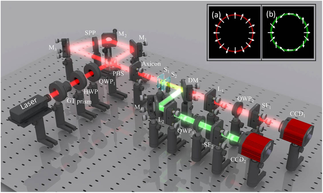
Fig. 1. Schematic of the experimental setup. GT prism, Glan–Taylor prism; HWP, half wave plate; QWP 1 QWP 2 QWP 3 M 1 M 2 M 3 M 4 S 1 S 2 MgO : LiNbO 3 L 1 L 2 f = 200 mm SF 1 SF 2 CCD 1 CCD 2
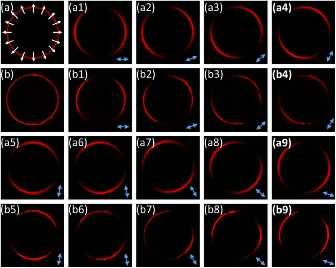
Fig. 2. (a) and (b) The simulated and experimental intensity distributions of the FF PV beams with TC l = 1
Fig. 3. (a) and (b) The simulated and experimental intensity distributions of the PV beams at the SH waveband. (a1)–(a9) Simulated intensity profiles of the generated PV beams when the GT prism has different polarization angles (0°, 20°, 40°, 60°, 80°, 100°, 120°, 140°, 160°) with respect to the positive horizontal direction. (b1)–(b9) are the corresponding experimental results.
Fig. 4. First and third rows are, respectively, the experimental results of the FF PV beams with δ / 2 + 2 γ = π / 3 δ / 2 + 2 γ = 2 π / 3
Fig. 5. Radii of the generated PV beams in the FF (left) and SH (right) wavebands with different TC.

Set citation alerts for the article
Please enter your email address
© Copyright 2018-2021 | Chinese Laser Press. All Rights Reserved 沪ICP备15018463号-20