
Fabrizio Consoli, Vladimir T. Tikhonchuk, Matthieu Bardon, Philip Bradford, David C. Carroll, Jakub Cikhardt, Mattia Cipriani, Robert J. Clarke, Thomas E. Cowan, Colin N. Danson, Riccardo De Angelis, Massimo De Marco, Jean-Luc Dubois, Bertrand Etchessahar, Alejandro Laso Garcia, David I. Hillier, Ales Honsa, Weiman Jiang, Viliam Kmetik, Josef Krása, Yutong Li, Frédéric Lubrano, Paul McKenna, Josefine Metzkes-Ng, Alexandre Poyé, Irene Prencipe, Piotr Ra?czka, Roland A. Smith, Roman Vrana, Nigel C. Woolsey, Egle Zemaityte, Yihang Zhang, Zhe Zhang, Bernhard Zielbauer, David Neely. Laser produced electromagnetic pulses: generation, detection and mitigation[J]. High Power Laser Science and Engineering, 2020, 8(2): 02000e22
- High Power Laser Science and Engineering
- Vol. 8, Issue 2, 02000e22 (2020)
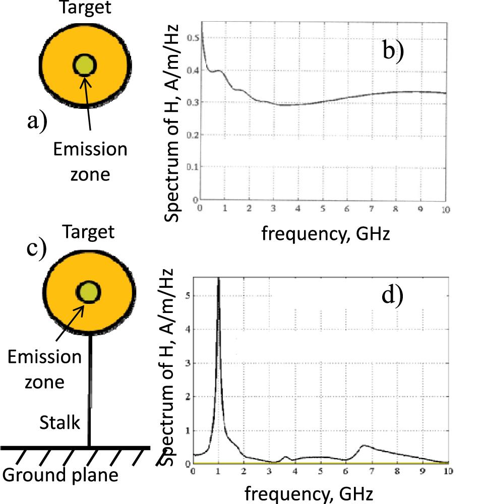
Fig. 1. Schematic of charged target (a) standing alone and (c) connected to the ground. Spectra of EMP emission (b) from the free standing target and (d) from the target connected to the ground.
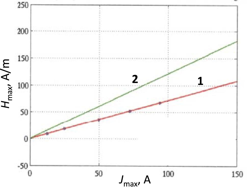
Fig. 2. Dependence of the radiated magnetic field at distance  cm from the antenna shown in Figure
 1 (c) on the current in the stalk: 1 – calculated numerically and 2 – evaluated from Equation (4 ).
cm from the antenna shown in Figure Fig. 3. Scheme of target charging in the case of short-pulse interaction with a thick solid target. Hot electrons are created in the laser focal spot (red zone). They spread in the target over a distance comparable to the mean free path (gray zone). The electrons escaping in vacuum create a spatial charge and prevent low-energy electrons from escaping. Electrons with energies higher than the surface potential escape from the target and create a net positive charge at the surface. Reprinted with permission from Ref. [13]. Copyright 2014 by the American Physical Society.
Fig. 4. Dependence of the target charge  on the laser energy and the pulse duration for the laser spot radius of
  , the absorption fraction
  and laser wavelength of
  . The dashed white rectangle shows the domain explored in the experiment. Reprinted with permission from Ref. [60]. Copyright 2015 by the American Physical Society.
on the laser energy and the pulse duration for the laser spot radius of , the absorption fraction and laser wavelength of . The dashed white rectangle shows the domain explored in the experiment. Reprinted with permission from Ref. [60]. Copyright 2015 by the American Physical Society. Fig. 5. Target charge  in nC calculated from the model as a function of the absorbed laser energy and the focal spot diameter for the pulse duration of 1 ps, wavelength
  and an insulated and laser size target. There is an optimal spot diameter for the target charging.
in nC calculated from the model as a function of the absorbed laser energy and the focal spot diameter for the pulse duration of 1 ps, wavelength and an insulated and laser size target. There is an optimal spot diameter for the target charging. Fig. 6. Target charge  in nC calculated from the model as a function of the absorbed laser energy and the target diameter for the pulse duration of 1 ps, the focal spot diameter of
  , wavelength of
  and an insulated target. There is a threshold on the target diameter below which the target charging becomes dependent on it.
in nC calculated from the model as a function of the absorbed laser energy and the target diameter for the pulse duration of 1 ps, the focal spot diameter of , wavelength of and an insulated target. There is a threshold on the target diameter below which the target charging becomes dependent on it. Fig. 7. (a) Time dependence of the current density of electrons emitted backward from the target surface at different distances from the laser axis obtained in the Monte Carlo simulation. (b) Time dependence of the electric current of escaped electrons collected at a distance of 1 mm from the target. Three simulations with the target radii 2.5, 5 and 7.5 mm are shown. The dashed line shows the ejection current obtained from the Monte Carlo simulation. Reprinted with permission from Ref. [13]. Copyright 2014 by the American Physical Society.
Fig. 8. (a) Simulation of the current at the bottom of the target assembly. Calculation with the SOPHIE code: the target radius is 5 mm, the laser pulse energy is 80 mJ and the pulse duration is 50 fs. The current is collected at an effective  resistance. (b) Comparison of the calculated waveform (red solid line) with the experimental data (blue dots). Reprinted with permission from Ref. [13]. Copyright 2014 by the American Physical Society.
resistance. (b) Comparison of the calculated waveform (red solid line) with the experimental data (blue dots). Reprinted with permission from Ref. [13]. Copyright 2014 by the American Physical Society. Fig. 9. Scheme of the field induced due to charge deposition on one plate of a capacitor–collector setup. The system is initiated by a flow of energetic particles from a pulsed laser-driven source. Reprinted from Ref. [73] under Creative Commons license .
Fig. 10. Top-view scheme of the vacuum chamber; the laser (red beam) is focused on a thin-foil target by an off-axis parabola mirror. Reprinted from Ref. [73] under Creative Commons license .
Fig. 11. (a)  signal detected by the D-dot probe in shot
  ; (b) time-gated normalized spectrogram of the signal. The origin of the timescale was set at the moment when the EMP signal reaches the D-dot probe. Reprinted from Ref. [73] under
 Creative Commons license .
signal detected by the D-dot probe in shot ; (b) time-gated normalized spectrogram of the signal. The origin of the timescale was set at the moment when the EMP signal reaches the D-dot probe. Reprinted from Ref. [73] under Fig. 12. (a) Component of the electric field normal to the D-dot ground plane measured in shot #29. (b) Comparison of several single-shot measurements of the electrical field component normal to the D-dot ground plane.
Fig. 13. Comparison between experimental D-dot measurements from shot #29 and PIC simulations of electric fields at the D-dot position, in the  and
and  directions. The origin of the timescale is here set at the moment of laser–target interaction, and the #29 measurement was thus time-shifted, with respect to Figures
 11 and 12 , by the EMP propagation time from target to D-dot probe. Reprinted from Ref. [73] under Creative Commons license .
and directions. The origin of the timescale is here set at the moment of laser–target interaction, and the #29 measurement was thus time-shifted, with respect to Figures Fig. 14. Examples of time-domain signals measured with Antennas (a) 1 and (b) 2 for shot  inside the vacuum chamber of the ABC facility and (c), (d) the corresponding amplitude envelopes obtained from Equation (
10 ). See Table 3 in Section 2.7.2 for further details. Reprinted with permission from Ref. [83]. Copyright 2015 by the IEEE.
inside the vacuum chamber of the ABC facility and (c), (d) the corresponding amplitude envelopes obtained from Equation (Fig. 15. Antenna waveforms from a Vulcan shot #13. Reprinted with permission from Ref. [9]. Copyright 2004 by the American Institute of Physics.
Fig. 16. Integrated waveform and FFT of signals shown in Figure 15 . Reprinted with permission from Ref. [9]. Copyright 2004 by the American Institute of Physics.
Fig. 17. Frequency spectra of the EMP measured from (a) the north–south and (b) east–west electro-optical probes. (c) Spectrum for signal detected by D-dot probe. Harmonics corresponding to those theoretically expected in chamber and listed in Table 1 are outlined by dashed red vertical lines. Reprinted from Ref. [90] under Creative Commons license .
Fig. 18. Time–frequency analysis of two laser shots. Multiple scanning window sizes have been applied of 100, 50 and 25 ns with transition to the smaller window sizes occurring at 80 and 320 MHz. The laser energy on target was 38 J for (a) and 365 J for (b). For both panels, the color scale represents the amplitude normalized to the scanning window length. The insets in each figure show frequency and time ranges of interest from the main figures. The axes in the insets have the same units as the main figures with the two insets for (b) sharing the same time axis.
Fig. 19. COMSOL 3D electromagnetic simulations of a cavity with four conducting cylinders inserted and connected to it. (a) Cavity scheme. Electric field distribution for the mode with resonance frequency of (b) 480.3 MHz; (c) 108.6 MHz; and (d) 175.7 MHz. The red arrows indicate the electric field directions; their size and length are associated with the relative field intensity. Reprinted with permission from Ref. [77]. Copyright 2015 by Elsevier B.V.
Fig. 20. Modulus of the single-sided Fourier spectrum of signals detected by the three antennas WM inside, SWB inside and WM outside for the shot  at ABC laser. The vertical dotted lines are the first 15 resonance frequencies for the modes of the hollow cavity. Reprinted with permission from Ref. [77]. Copyright 2015 by Elsevier.
at ABC laser. The vertical dotted lines are the first 15 resonance frequencies for the modes of the hollow cavity. Reprinted with permission from Ref. [77]. Copyright 2015 by Elsevier. Fig. 21. Shot #1525: FFT and normalized spectrograms for the signals acquired by Antennas 1 and 2 inside the chamber. Reprinted with permission from Ref. [83]. Copyright 2015 by the IEEE.
Fig. 22. Distribution of the magnetic induction in arbitrary units inside the target chamber at the fundamental resonant frequency of 287 MHz. The field is distorted by the presence of the input glass window (left), focusing lens and metallic lens holder, target holder system (right) and a metal plate (bottom). Reprinted with permission from Ref. [96]. Copyright 2016 by the Institute of Physics.
Fig. 23. Tridimensional distribution of the electric field inside the PALS vacuum chamber at the frequency of 402 MHz. Reprinted from Ref. [95] with permission. Copyright 2018 by ENEA.
Fig. 24. Space distribution of the time derivative of the magnetic flux calculated at the resonant frequency of 287 MHz in the PALS chamber (in arbitrary units) equipped with basic items. Reprinted with permission from Ref. [96]. Copyright 2016 by the Institute of Physics.
Fig. 25. (a) ELISE nozzle sketch; (b) diagnostic arrangement in the PALS vacuum chamber. FSI: three-frame interferometer, IC: ion collector, A1 and A2: positions of B-dot antennas in the target chamber. Reprinted with permission from Ref. [98]. Copyright 2017 by the American Institute of Physics.
Fig. 26. The FFT of typical signals detected by the probes A1 and A2 shown in Figure 25 (b). Frequencies corresponding to the nozzle shielding housing, eigenfrequency of the spherical vacuum chamber free of accessories and laser pulse duration  are shown by colored cross-hatched marks. Gray zone shows the oscilloscope background noise. Reprinted with permission from Ref. [98]. Copyright 2017 by the American Institute of Physics.
are shown by colored cross-hatched marks. Gray zone shows the oscilloscope background noise. Reprinted with permission from Ref. [98]. Copyright 2017 by the American Institute of Physics. Fig. 27. (a) Waveforms of the voltages detected by Antenna  for the 300 J, 1 ps and 100 J, 10 ps laser pulses at the SG-II-UP laser and (b) their corresponding frequency spectra.
for the 300 J, 1 ps and 100 J, 10 ps laser pulses at the SG-II-UP laser and (b) their corresponding frequency spectra. Fig. 28. Dependence of the radiated EMP power on the laser energy.
Fig. 29. Simulated distribution of the radiated field amplitude at (a) 1.0, (b) 3.5, (c) 21 and (d) 60 ns. The arrows on the wavefronts in (a)–(d) indicate the corresponding power flow direction. The electric field waveforms at the positions  ,
,  and
and  are illustrated in Figure
 30 (a).
, and are illustrated in Figure Fig. 30. (a) The electric fields at the positions  ,
,  and
and  and (b) their corresponding frequency spectra.
, and and (b) their corresponding frequency spectra. Fig. 31. Two Möbius antennas perpendicular to each other to measure two components of the laser-induced EMP.
Fig. 32. (a) Oscilloscope traces of an EMP signal detected by two Möbius loop antennas for a laser shot on a  thick titanium foil. The laser energy was 3 J. (b) Corresponding frequency spectra. The blue and green curves show the signals measured parallel and perpendicular to the laser polarization, respectively.
thick titanium foil. The laser energy was 3 J. (b) Corresponding frequency spectra. The blue and green curves show the signals measured parallel and perpendicular to the laser polarization, respectively. Fig. 33. Functional scheme of contributions for the stored signal in EMP measurements.
Fig. 34. Experiment performed at PALS laser in Prague. (a) Typical shot on graphite target; (b) similar shot but with cables detached from the oscilloscope: measurement of background noise. Reprinted from Ref. [95] with permission. Copyright 2018 by ENEA.
Fig. 35. (a) HSD-2B(R) and HSD-4A(R) D-dot sensors. Reprinted with permission from Ref. [118]. Copyright 1986 by Springer. (b) Prodyn AD-80(R) ACD D-dot sensor. (c) PPD-1A(R) E sensor (exploded view). Reprinted with permission from Ref. [118]. Copyright 1986 by Springer.
Fig. 36. (a) Typical configuration of the magnetic field sensors  Multi-Gap Type Free-Field Models, of the type supplied by Prodyn[76]. (b) Scheme of the Möbius loop magnetic field sensor. Reprinted with permission from Ref. [88]. Copyright 1974 by IEEE. (c) Typical configuration of cylindrical Möbius loop sensors[118, 133]. Reprinted with permission from Ref. [133]. Copyright 1978 by IEEE.
Multi-Gap Type Free-Field Models, of the type supplied by Prodyn[76]. (b) Scheme of the Möbius loop magnetic field sensor. Reprinted with permission from Ref. [88]. Copyright 1974 by IEEE. (c) Typical configuration of cylindrical Möbius loop sensors[118, 133]. Reprinted with permission from Ref. [133]. Copyright 1978 by IEEE. Fig. 37. (a) Sketch of the experimental setup and (b) target currents neutralizing massive (5 mm thick) copper target irradiated with the PALS and KrF lasers delivering intensities of  and
and  , respectively. The duration of the KrF laser was 23 ns and of the PALS laser was 400 ps. Reprinted with permission from Ref. [136]. Copyright 2019 by the SPIE.
and , respectively. The duration of the KrF laser was 23 ns and of the PALS laser was 400 ps. Reprinted with permission from Ref. [136]. Copyright 2019 by the SPIE. Fig. 38. Target current observed with the use of a 0.056  resistor probe inserted in the target holder system. The inset shows a detail of the target current modulated with frequencies associated with the generated EMP.
resistor probe inserted in the target holder system. The inset shows a detail of the target current modulated with frequencies associated with the generated EMP. Fig. 39. Application of the inductive probe for the target current flow measurement. (a) Photo of an inductive target double probe. (b) View of the target holder system equipped with the inductive probe. The loops are localized inside the groove. The copper cylinder avoids the loop picking up the EMP, which is produced within the target chamber.
Fig. 40. Typical current waveform neutralizing the target charge; the inset: oscillogram trace rescaled to  , where
  is the output voltage on the inductive target probe. Polyethylene target was exposed to laser pulse intensity of
  . Reprinted with permission from Ref. [55]. Copyright 2017 by the IoP.
, where is the output voltage on the inductive target probe. Polyethylene target was exposed to laser pulse intensity of . Reprinted with permission from Ref. [55]. Copyright 2017 by the IoP. Fig. 41. Measurement of the  scattering parameter for the 10 m RG58 coaxial cable and inferred curves of
  for RG58 cables of different lengths. The
  function, with
  in gigahertz units, is also shown as a reference. Reprinted from Ref. [95] with permission. Copyright 2018 by ENEA.
scattering parameter for the 10 m RG58 coaxial cable and inferred curves of for RG58 cables of different lengths. The function, with in gigahertz units, is also shown as a reference. Reprinted from Ref. [95] with permission. Copyright 2018 by ENEA. Fig. 42. Shot on Au target enriched with H and B, when long RG58 cables are used on SWB (70 m) and MONO (102 m) antennas inside the chamber. Reprinted from Ref. [95] with permission. Copyright 2018 by ENEA.
Fig. 43. (a) Comparison between signals from SWB and MONO antennas for shot #45992. (b) Comparison of the SWB antenna signal for shot #45992 with the neutralization current measured by the inductive current probe for the same and also for other shots. Reprinted from Ref. [95] with permission. Copyright 2018 by ENEA.
Fig. 44. Scheme of the experiment in the two configurations represented by shots  and
and  (
( ). Reprinted from Ref. [94] under
 Creative Commons license .
and (). Reprinted from Ref. [94] under Fig. 45. Scheme of the electro-optic probe. Reprinted from Ref. [94] under Creative Commons license .
Fig. 46. Measured electric field component  for shots (a) #1590 and (b) #1597. Reprinted from Ref. [94] under
 Creative Commons license .
for shots (a) #1590 and (b) #1597. Reprinted from Ref. [94] under Fig. 47. Measurement of  in shot #1590 and
  in shot #1597, with related simulations for
  . Reprinted from Ref. [94] under
 Creative Commons license .
in shot #1590 and in shot #1597, with related simulations for . Reprinted from Ref. [94] under Fig. 48. Layout of the optical EMP diagnostic in the Vulcan Petawatt interaction chamber. Only the east–west and north–south probes (EWP and NSP) were used, with crystals 1.25 m from the TCC. Reprinted from Ref. [90] under Creative Commons license .
Fig. 49. (a) Cartesian coordinate plot depicting the location of the KDP crystals within the chamber. The origin is defined here as the bottom north–east corner of the Vulcan Petawatt interaction chamber. The TCC where targets were located is also shown for comparison. (b) Simplified schematic of the crystal mounts, where the middle two aluminum layers enable fine adjustment and the plastic insulates the crystals from surrounding metals. Reprinted from Ref. [90] under Creative Commons license .
Fig. 50. Temporal electric field behavior (a) calculated using the raw voltage data and (b) with a low-pass frequency filter applied to remove high-frequency electrical noise, and the contribution to the initial peak by optical self-emission coupled into the optical fibers subtracted. The time axes have been shifted such that  corresponds to the arrival of the 227 TW drive laser pulse on target. Reprinted from Ref. [90] under
 Creative Commons license .
corresponds to the arrival of the 227 TW drive laser pulse on target. Reprinted from Ref. [90] under Fig. 51. Electro-optic setup fielded on Cerberus laser. Reprinted from Ref. [148] under Creative Commons license .
Fig. 52. (a) Experimental setup for the investigation of EMP using proton probing. (b)–(d) Snapshots of a pulse of electric current propagating along a folded wire toward ground. Snapshot times are given by the TOF of protons from the source to the interaction region. Arrows in panels (b) and (c) show the direction of the current. Dotted lines show the deflection of protons from the local field. For the late probing time in (d), the electromagnetic field is weak. The black region encircled by the dotted lines indicates the spatial extent of proton beam. Reprinted with permission from Ref. [68]. Copyright 2018 by the American Institute of Physics.
Fig. 53. (a) Experimental layout for the femtosecond electron deflectometry measurement. Fast electrons propagating across the wire are detected by a stack of imaging plates. (b) Time traces of the beam deflection in the transverse direction. Reprinted from Ref. [50] under Creative Commons license .
Fig. 54. (a) Normalized peak electric and magnetic field strength plotted as a function of laser energy. Measurements were taken using the D-dot and B-dot east probes. The red dashed line represents the best fit to the probe data, using a square root function of laser energy. (b) Normalized peak magnetic field strength divided by the square root of on-target energy is plotted in black for a variety of laser pulse durations (B-dot east probe). Shown in red is the number of emitted electrons (measured by an electron spectrometer) divided by the on-target laser energy. B-dot data is divided by the square root of the laser energy to account for the energy dependence of EMP presented in panel (a). Intensity ranges from  to
to  .
.
to . Fig. 55. Normalized peak electric field strength plotted as a function of laser energy for wire, flag and rectangular foil targets (D-dot east probe). Laser focal intensity ranges from  to
to  . Note how changing the wire diameter has led to a deviation from the relationship between EMP and on-target laser energy established in Figure
 54 (a).
to . Note how changing the wire diameter has led to a deviation from the relationship between EMP and on-target laser energy established in Figure Fig. 56. (a) Three different stalk designs: 1 – standard cylindrical geometry, 2 – sinusoidally modulated stalk with the same maximum cross section as the standard cylinder, 3 – spiral stalk design with an identical diameter to 1. (b) Normalized peak electric field strength plotted as a function of laser energy for aluminum and CH stalks with cylindrical, spiral and sinusoidal geometries. Data is taken from the D-dot east probe and presented as a fraction of the peak electric field for the aluminum stalk. Laser focal intensity varies between  and
and  .
.
and . Fig. 57. Dependence of EMP energy on laser energy in experiments with gold targets of thickness varying from 10 and 125  . All targets were mounted on 60 mm long, 1 mm diameter quartz glass stalks. Linear fits to the data show a slope variation of less than 20% between the different thickness targets, and an averaged fit to all the datasets is shown.
. All targets were mounted on 60 mm long, 1 mm diameter quartz glass stalks. Linear fits to the data show a slope variation of less than 20% between the different thickness targets, and an averaged fit to all the datasets is shown. Fig. 58. EMP energy generated by hemispherical targets mounted on 23 mm long, 1 mm diameter glass and carbon fiber stalks, showing lower overall emissions for higher resistivity stalks, as expected. Linear trend lines with drive laser energy have been fitted to the data.
Fig. 59. Dependence of EMP energy on target dimension for thin 0.01–0.125 mm gold foils mounted on glass stalks, fitted with a linear trend line. To compare the EMP energy per joule for differently shaped round and rectangular targets, the square root of target area has been used as an equivalent ‘length’ dimension. The error bars are the standard deviation observed over many shots for each target size.
Fig. 60. Dependence of the (a) normalized electric field energy and (b) magnetic energy on the target diameter. Red dots – experimental data, solid lines – results of simulations with ChoCoLaT2 code[36]. The targets were  thick tantalum foils of varying transverse sizes mounted on 25 mm long, 3 mm wide plastic stalks.
thick tantalum foils of varying transverse sizes mounted on 25 mm long, 3 mm wide plastic stalks. Fig. 61. (a) Vacuum test chamber used for vacuum trapping of oil micro-droplets. (b) A view of the loaded vacuum trap (under vacuum) without the imaging optics in place. The trapped droplet (small, bright spot at the center of the image) is clearly visible. Reprinted with permission from Ref. [159]. Copyright 2015 by the American Institute of Physics.
Fig. 62. Schematic of the target chamber, alignment and diagnostic layout for the high-intensity laser droplet interaction experiments. Viewing angles were established to monitor the trapped droplet position (Sumix cameras [A] and [B]) and also for accurate alignment with the main heating beam under vacuum (CCD camera [C]). Reprinted with permission from Ref. [159]. Copyright 2015 by the American Institute of Physics.
Fig. 63. Radiofrequency emission measurements from a high-intensity laser-irradiated droplet ((a) and (b)) and carbon wire ((c) and (d)) interaction. The droplet background and shot measurements record a small early time noise signal from a switched Pockels cell firing with the main laser, followed by an EMP pulse generated by the laser–target interaction. Reprinted with permission from Ref. [159]. Copyright 2015 by the American Institute of Physics.
Fig. 64. Schematic view of the ‘birdhouse’ EMP mitigation concept. Reprinted with permission from Ref. [164]. Copyright 2018 by the American Institute of Physics.
Fig. 65. EMP mitigation ratio for the ‘birdhouse’ scheme as a function of frequency. Data from two B-dot probes and Möbius loop are shown. Reprinted with permission from Ref. [164]. Copyright 2018 by the American Institute of Physics.
Fig. 66. (a) Photo of a target mounted on an inductive–resistive holder to mitigate the EMP emission. (b) Photo of a target mounted on a resistive holder in the LULI2000 experiment.
Fig. 67. (a) Discharge current intensity and (b) total ejected charge as a function of time for the reference holder (1) and the new holder (2).
Fig. 68. (a) Time dependence of the magnetic field measured by B-dot at a distance of 54 cm from the TCC: red – conducting holder, green – inductive–resistive holder. (b) Frequency-dependent mitigation factor: ratio of the magnetic fields measured by the resistive and conducting holders.
Fig. 69. System of four B-dot probes developed for EMP measurements in LMJ–PETAL experiments.
Fig. 70. Photo of the target used in the combined LMJ–PETAL shots. The target holder is horizontally oriented in the chamber.
Fig. 71. (a) Representative oscilloscope signals measured inside (blue) and outside (green) a 2 mm thick protective aluminum shielding with 3 J on a  titanium target. (b) Fourier transform of the signals shown in panel (a).
titanium target. (b) Fourier transform of the signals shown in panel (a). Fig. 72. Energy scaling of the integrated EMP signal inside and outside the 2 mm thick aluminum shielding.
Fig. 73. (a) Detailed structural model used for an EMP propagation simulation, including the P3 interaction chamber and beam transport manifold with TMEs. Ports of interest are indicated by marks P1–P4; AHO indicates the location of the absorber cladding. (b) Electric field snapshot at a time of 75 ns in the central horizontal plane of a vacuum system for the laser energy 2 kJ and conversion efficiency to primary EMP of 1%.
Fig. 74. Maxima of the electric field amplitude observed at selected ports in a simulation with a laser energy of 2 kJ and conversion efficiency to EMP of 1%. Values at different ports are distinguished by colors. Ports are indicated in the structural model (Figure 73 (a)) by marks P1 – orange, P2 – blue, P3 – green and P4 – red. See text for more detailed explanation.
Fig. 75. Compilation of the measured amplitudes of EMP signals at different laser installations. Field values present in this picture were taken or estimated by Refs. [52, 60, 71, 73, 90, 94, 178], from data shown in this paper or supplied by private communications or reports. Blue and red zones outline the data obtained with ps and ns laser pulses, respectively. All data were normalized to the reference distance of 1 m from the source. Values for the ABC[94] and the XG-III[71] experiments were obtained at distances 85 mm and 400 mm from the target, respectively. The normalization might produce a field overestimation of a few times.
|
Table 1. Values of different parameters calculated for the fundamental modes of Vulcan Petawatt chamber.
| ||||||||||||||||||||||||||||||||||
Table 2. Frequencies of the expected harmonics and detected spectral peaks in the Vulcan experiment. Superscript E-W or N-S indicates the mode axis and numbers 1, 2 and 3 indicate the harmonic order.
|
Table 3. Laser energy and intensity, target thickness, and the measured energy and peak–peak amplitude of detected signals for two shots on the ABC facility.
|
Table 4. EMP energy flow at the selected ports during  calculation in percentage of initial EMP energy for different absorbers. See text for explanation of abbreviations.
calculation in percentage of initial EMP energy for different absorbers. See text for explanation of abbreviations. 
Set citation alerts for the article
Please enter your email address
© Copyright 2018-2021 | Chinese Laser Press. All Rights Reserved 沪ICP备15018463号-20