
Haochen Li, Tianyuan Liu, Yuchao Fu, Wanxiang Li, Meng Zhang, Xi Yang, Di Song, Jiaqi Wang, You Wang, Meizhen Huang. Rapid classification of copper concentrate by portable laser-induced breakdown spectroscopy combined with transfer learning and deep convolutional neural network[J]. Chinese Optics Letters, 2023, 21(4): 043001
- Chinese Optics Letters
- Vol. 21, Issue 4, 043001 (2023)
Abstract
Keywords
1. Introduction
Flotation concentrates contain a variety of elements, which directly affect their economic value. For example, the copper content directly determines the price of the copper concentrate. Other impurities, such as Fe, Zn, Pb, and S, will increase the cost of smelting and be harmful to the environment[1]. Therefore, it is urgent to develop a portable and rapid detection technology for the in situ measurement of bulk copper concentrates.
Traditional analytical methods applied in the elemental analysis of flotation concentrates require a series of time-consuming and laborious sample pretreatments, resulting in high costs[2]. Laser-induced breakdown spectroscopy (LIBS) is an elemental analysis method. A laser beam is focused on the sample surface to produce plasma. The spectrum of the plasma can be used to characterize the elements contained in the analyte and quantitative information[3], with the advantages of being fast, microdestructive, no sample pretreatment, in situ and multielement simultaneous analysis[4]. LIBS is of wide interest in many fields such as geology, coal quality analysis, metal recovery, environmental protection, and health care[5–9]. Therefore, LIBS has great potential in the application of rapid classification of flotation concentrates.
The physical properties of concentrate samples vary with different batches and mining areas. Therefore, the measurement is easily affected by matrix effects, which interfere with the detection of some trace elements[10]. As a result, the accuracy of classification is reduced. There is serious instability in the temporal evolution of the laser-induced plasma, resulting in poor reproducibility of LIBS spectra[11]. Considering the need for rapid applications, portable LIBS systems have to be compact in size. Some aspects (spectral resolution, spectral range, laser energy, temporal resolution) of the portable LIBS system are not as advanced as those of benchtop LIBS systems, which further decreases the accuracy in classifying mineral samples[12]. In response to the above problems, most studies adopted advanced machine-learning models [K-nearest neighbor (KNN), support vector machine (SVM), random forest (RF), backpropagation neural network (BPNN)] to process LIBS spectral data, which reduces spectral random noise and corrects the interference of matrix effects, thereby improving classification accuracy[13–15]. However, the performance of the above models depends on feature selection methods. Different feature selection methods have their own limitations and require a strong knowledge of physics and spectral data processing[16].
Sign up for Chinese Optics Letters TOC. Get the latest issue of Chinese Optics Letters delivered right to you!Sign up now
As a branch of machine learning, deep learning can automatically extract the features in one pass, which greatly simplifies the workflow of machine learning[17]. In addition, deep learning is considered adept at correcting the interference of multiple factors[18]. Therefore, it is currently attracting more and more researchers’ interest. Convolutional neural networks (CNNs) are one of the most widely used deep-learning models. Chen et al. used a self-designed CNN to classify 119 rock samples from five classes. They compared 1D-CNN with 2D-CNN and found the classification accuracy of 2D-CNN was higher[17]. Li et al. achieved a high-accuracy classification of geological samples by employing a CNN with five convolutional layers and two pooling layers. Their spectra were collected by MarSCoDe during preflight testing[18]. Zhao et al. developed a 1D-CNN model to classify iron ore, and for the first time interpreted the effectiveness of the CNN model by the t-distributed symmetric neighbor embedding algorithm (t-SNE)[19].
In general, increasing the depth of the CNN model is an effective approach toward increasing the performance of the model[20]. At present, most of the existing studies on CNN and LIBS designed their own convolutional structures with a small number of convolutional layers (typically 2–5 layers, due to the limited sample number), which are unable to compare to the deep CNN (typically more than 100 layers, trained with millions of data)[17–19]. Moreover, the design of the CNN model structure is usually based on experience and is time-consuming and laborious. Training the deep CNN model from scratch would require millions of data to achieve the desired accuracy. This data amount is impossible for LIBS research. To address these issues, we introduce the concept of transfer learning. Transfer learning aims to apply previously learned knowledge (source domain) to solve new problems (target domain). It achieves better performance and saves training time in a target domain that has a small amount of data with the help of the knowledge learned from the source domain that has sufficient training data[21–23]. One of the practices of transfer learning is to set the pretraining weights trained with sufficient data as initialization weights of the model and then train the model for a second time with data from the target domain. This approach is also known as fine-tuning of the model[24].
This paper explored the feasibility of applying the pretrained CNN model to a portable LIBS system to classify copper concentrates via transfer learning without the need for redesigning the CNN structure. The spectra of 11 classes of copper concentrates were obtained using a self-developed portable LIBS device. Four pretrained CNN models were tried, including VGG16, ResNet18, DenseNet121, and InceptionV3. To demonstrate the performance of CNN models and transfer learning in copper concentrate classification, other machine-learning models, feature selection, and dimension reduction methods were also tried [principal component analysis-BPNN (PCA-BPNN), PCA-SVM, Chi-square test-BPNN (CST-BPNN), and CST-SVM]. The results showed that the performance of the CNN models was higher than that of traditional machine-learning models. This study shows the great potential of the deep CNN model and transfer learning in the classification of copper concentrates by portable LIBS, which can open the way for the accurate classification of LIBS spectra of substances with similar chemical compositions.
2. Experiments
2.1. LIBS equipment
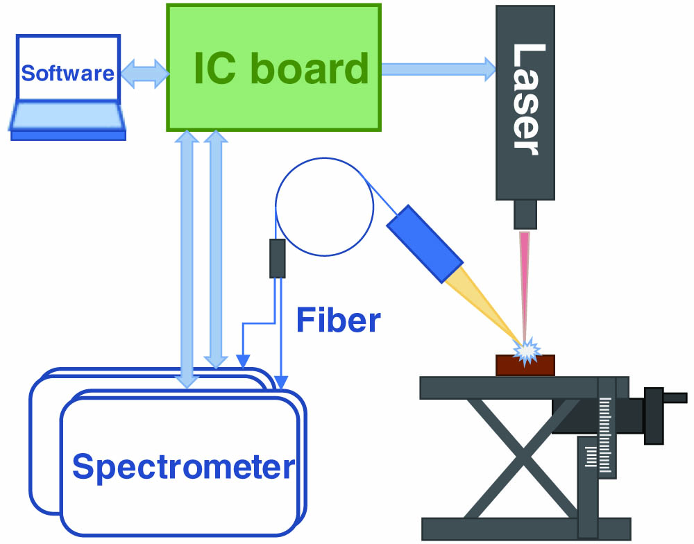
The block diagram of the self-developed portable LIBS device is shown in Fig. 1. The excitation source was a 1064 nm diode-pumped solid-state (DPSS) laser (actively -switched Nd:YAG, 10 µJ/pulse, 10 ns pulse duration, 8 kHz repetition rate, power fluctuation ). The focused spot diameter is 10 µm. The plasma emission spectra were collected by two self-designed Czerny-Turner spectrometers with wavelengths ranging from 252 to 373 nm and 445 to 550 nm, with a resolution of 0.1 to 0.2 nm, equipped with a 2048-pixel linear CCD[25,26].
![]()
Figure 1.Block diagram of portable LIBS setup.
2.2. Experiment
The copper concentrate samples were provided by Zijin Mining Group Co., Ltd. (Fujian, China). They were sampled from different batches of bulk copper concentrate by a Zijin copper smelter. We named them #1–#10 in this paper. The copper content of the samples was determined by the iodometric method by analytical testers of Zijin Mining Group Co., Ltd. We purchased a copper concentrate standard material ZBK338C, named #11 in this paper. The copper content of all 11 samples is described in Table 1. The copper concentrate was weighed (about 0.2 g) and pressed into a pellet under a pressure of 6 MPa for 120 s. Each copper concentrate sample was pressed into three pellets. Forty spectra were obtained at different positions of each pellet, and a total of spectra were obtained for each class. A total of spectra were obtained. The laser repetition rate was 8 kHz. The CCD exposure time was set to 65 ms. In this setup, a spectrum was the accumulation of the plasma generated by 520 laser pulses. To obtain a higher signal-to-noise ratio, the pellets were kept moving during the measurement. Typical LIBS profiles of copper concentrate pellets obtained by the portable LIBS system are shown in Fig. 2. Considering the need for rapid detection, each spectrum obtained at different locations on the pellets was considered an independent spectral sample in this paper.
![]()
Figure 2.Typical spectrum of copper concentrate acquired by portable LIBS apparatus.
| No. | 1 | 2 | 3 | 4 | 5 | 6 | 7 | 8 | 9 | 10 | 11 |
|---|---|---|---|---|---|---|---|---|---|---|---|
| Mass fraction (%) | 18.86 | 19.68 | 20.58 | 21.80 | 22.49 | 23.66 | 24.42 | 25.52 | 26.21 | 27.73 | 27.62 |
Table 1. Copper Contents of the Copper Concentrate Samples
3. Data Analysis
3.1. CNN classification model
CNN consists of convolutional layers, pooling layers, and fully connected layers. The convolution layer shares the same weights in all the subareas of the input matrix. Therefore, the CNN model can comprise many convolution layers without the computation cost exploding. Convolutional layers have strong feature extraction capabilities, so CNN requires less data preprocessing than BPNN. In a deep CNN model, the earlier convolutional layer extracts more detailed and small-sized features, and the later convolutional layers extract more macroscopic and large-scale features.
We tried four publicly available and most successful CNN models (VGG16, ResNet, DenseNet, and InceptionNet) for transfer learning. The models were trained on ImageNet and achieved high classification accuracy[27]. The ImageNet is a benchmark data set in machine vision that spans 1000 object classes and contains 1,281,167 training images[28].
VGG: The VGG network is the first CNN model that effectively improves performance by increasing the depth; VGG16 only contains convolutional layers with convolution kernels and pooling layers. It solves the problem of AlexNet’s poor identification of detail features, laying the foundation for later deep CNNs[20].
ResNet: ResNet proposed the residual module to solve the problem of performance degradation after the depth exceeds a certain level and has an ultradeep network structure (more than 1000 layers)[29].
DenseNet: Compared with ResNet, DenseNet proposed a more aggressive dense connection mechanism: all layers are connected. Another major feature of DenseNet is feature reuse through the connection of features on channels. These features allow DenseNet to achieve better performance than ResNet with fewer parameters and computational costs[30].
InceptionNet: InceptionNet increases the width of the network, which is a different direction (horizontal) compared to the way in which VGG stacks convolutional layers (vertical). InceptionNet adopts the method of multidimensional convolution and reaggregation to widen the network structure and reduces the number of parameters through the 1 × 1 convolution operation, which has achieved better results[31].
All CNN constructions in this article are done in PyTorch 3.3.
3.2. Two other machine-learning models as comparison
BPNNs and SVMs are widely applied with LIBS and perform well with the complex analytes, but their performance is affected by the feature engineering[32]. PCA is a well-known unsupervised feature dimension reduction method that can alleviate the problem of the curse of dimensionality[33]. CST is a feature selection method for classification. By using individual CSTs, each independent variable is examined to see whether it is independent of the dependent variable. The smaller -value of the test statistic, the more correlated the independent variable is with the dependent variable; therefore it is an important feature[34].
3.3. Model performance evaluation
The overall discriminative classification ability of the model is measured by accuracy, which is the ratio of all correctly classified results to the total observed values in the data set. The calculation formula was as follows:
3.4. Deep CNN model retraining process
For model retraining, the last fully connected layer in the CNN model was replaced with a fully connected layer with 11 neurons for 11 classes of output. The training batch size and learning rate were optimized by the grid search method. After optimization, unified training parameters were applied for the four CNN models: the learning rate was 0.0001, the training batch size was 16, and the learning rate was multiplied by a factor of 0.5 every 7 epochs. In the following section of this paper, we compared three training processes that differ in details: (1) the convolutional layers were frozen and only the fully connected layers were trained; (2) the convolutional layers were unfrozen and both the convolutional and fully connected layers were trained; (3) both the convolutional and fully connected layers were trained from scratch with random initial weights.
4. Results and Discussion
4.1. LIBS profiles of copper concentrate and its pretreatment
Due to the low resolution of the portable spectrometer, the spectral lines are crowded. Moreover, the weak spectral lines of trace elements are interfered with by the strong spectral lines of the matrix elements (Cu, Fe, and Si) and cannot be observed. Due to the limited wavelength range, the spectral lines of elements such as Na and K are not in the spectral range. The only observable elements were Cu, Mg, Si, Fe, Zn, and Ca. Figure 3 shows the elemental line intensities of Cu, Ca, Zn, and Mg in the raw spectra of 11 copper concentrate samples. From Fig. 3, due to the severe matrix effect and self-absorption, the correlation between the spectral line intensity of Cu and the copper content was weakened. In these four elements, most of the standard deviations of the spectral line intensities were greater than the difference in the class average intensities. Therefore, using one or more spectral line intensities as the only basis for classification might lead to many misidentifications. PCA was performed on the raw spectra of 11 classes. The plots of the first three principal components are shown in Fig. 4. From Fig. 4, the spectra of #11 were clearly distinguished from other classes in the two-dimensional space of principal components 1 and 2. However, the spectra of the other 10 classes overlapped, which indicated that it was difficult to achieve high classification accuracy using PCA scores as the extracted features.
![]()
Figure 3.Elemental spectral line intensities of the raw spectra of copper concentrates from 11 classes.
![]()
Figure 4.PCA plot of the raw spectra of copper concentrates from 11 classes.
4.2. Model construction and optimization
2D-CNN requires data to be input in the form of matrices. The deep CNN models in PyTorch require a data size of because these models are pretrained with data of such size, and they would have the best performance on such size[27]. Therefore, we took the following steps to convert the data to a size of . We first zero-padded at the start and the end of the spectrum and increased the feature number from 4096 to 6272. Then the spectrum was folded into the dimension . Finally, through pixel copying, each row of the matrix was copied into 8 rows to obtain a matrix. The specific process is shown in Fig. 5. The spectrum folded into a 2D matrix is shown in Fig. 6.
![]()
Figure 5.Steps for conversion of 1D spectra to 2D matrix.
![]()
Figure 6.Schematic diagram of 2D spectrum (left) and 2D spectrum image (right).
The advantage of CNN is to automatically extract features, so the spectra were directly converted into the 2D matrices without any noise reduction and baseline correction.
We first freeze all the parameters of the convolutional layers and only perform the gradient descent update process on the weights of the fully connected layers. The performance of the four CNN models is shown in Table 2. From Table 2, the accuracies of the models were quite low, indicating that the features extracted by the CNN models in the task of machine-vision classification had a very limited effectiveness on the LIBS classification task. The reason may be that there are some differences between the pictures of animal/vehicle/person and the spectral matrices. For example, the spectral features are static, and the position of a certain spectral line is the same in all spectral matrices. Moreover, the shape of one spectral line may not be substantially different from the other[35].
| Model | Training Accuracy | Validation Accuracy | Test Accuracy |
|---|---|---|---|
| VGG16 | 73.4% | 82.2% | 79.9% |
| ResNet18 | 71.8% | 68.6% | 69.3% |
| DenseNet121 | 76.4% | 59.1% | 51.1% |
| InceptionV3 | 70.7% | 65.9% | 65.5% |
Table 2. Performance of the CNN Models with the Convolutional Layers Frozen and Only Fully Connected Layers Trained
We tried to unfreeze the parameters of the convolutional layers and perform the training process on all parameters of the model. The performance of the four models is shown in Table 3. The training process is shown in Fig. 7. The confusion matrices are shown in Fig. 8.
![]()
Figure 7.Training process of the four CNN models.
![]()
Figure 8.Confusion matrices of the four CNN models on the test set (two upper panels, VGG16 and ResNet18; two lower panels, DenseNet121 and InceptionV3).
| Model | Training Accuracy | Validation Accuracy | Test Accuracy |
|---|---|---|---|
| VGG16 | 99.7% | 95.1% | 96.2% |
| ResNet18 | 100% | 94.7% | 92.8% |
| DenseNet121 | 100% | 94.3% | 93.6% |
| InceptionV3 | 100% | 93.6% | 93.6% |
| NPT-VGG | 99.1% | 88.63% | 89.4% |
| NPT-ResNet | 100% | 85.2% | 83.3% |
| NPT-DenseNet | 100% | 62.1% | 61.4% |
| NPT-Inception | 100% | 80.7% | 81.1% |
Table 3. Performance of the CNN Model with the Convolutional Layer Unfrozen and Trained with All Parameters
From Table 3, in the case of unfreezing the convolutional layer, the four CNN models have obtained better classification accuracy, among which the accuracy of VGG16 was the highest, with 95.1% on the validation set and 96.2% on the test set.
We also tried to initialize the weights randomly rather than using pretrained weights, and found that the time cost for model training increased by dozens of times, and the test accuracy of all CNN models was below 90%, as shown in Table 3. Therefore, using pretrained weights greatly improves the training speed and the accuracy of CNN models in LIBS classification tasks. The result indicated that the features extracted by the CNN models in the task of machine vision were effective for the classification task of LIBS spectra to some extent.
4.3. Comparison with other machine-learning models
The PCA-BPNN, PCA-SVM, CST-BPNN, and CST-SVM models are constructed, respectively. The data sets were the same as 2D-CNN. The classification results of the four machine-learning models are shown in Table 4. These results were directly compared with those of CNN models, as shown in Fig. 9.
![]()
Figure 9.Comparison of classification accuracy between CNN models and traditional machine-learning models on the test set.
| Model | Training Accuracy | Validation Accuracy | Test Accuracy |
|---|---|---|---|
| PCA-BPNN | 100% | 92.5% | 91.3% |
| PCA-SVM | 98.7% | 89.8% | 85.2% |
| CST-BPNN | 100% | 92.4% | 90.5% |
| CST-SVM | 100% | 88.3% | 87.5% |
Table 4. Performance of the Four Machine-Learning Models
PCA reduced the feature dimension to 100 principal components as the input of PCA-BPNN and PCA-SVM. The CST selected 794 features as the input of CST-BPNN and CST-SVM. The scores of the selected features were significantly higher than those of background and noise. A schematic diagram of the features selected by the CST is shown in Fig. 10.
![]()
Figure 10.Schematic diagram of the spectral features selected by the CST methods.
The numbers of hidden layers and neurons of BPNN were optimized by the grid search method. BPNN with multiple layers showed little improvement compared to the single-layer BPNN. Therefore, we chose single layer as the optimal hidden layer number, and the number of nodes in the hidden layer was 100. The accuracy of PCA-BPNN on the test set was 91.60%. The accuracy of CST-BPNN was 90.5%.
For the SVM model, the grid search method was applied to optimize the penalty parameter and kernel function parameter. The optimized penalty parameter C is 0.1, and the kernel function parameter γ is 0.001. The accuracy of PCA-SVM on the test set was 85.2%, and the accuracy of CST-SVM was 87.5%.
5. Conclusion
In this study, portable LIBS technology combined with the pretrained CNN model and transfer learning was applied to accurately classify copper concentrate samples from 11 classes. The spectral lines of copper concentrate acquired by portable LIBS are crowded, with few detectable elements, and the reproducibility is not as good as that of desktop LIBS. To highlight the advantages of CNN models, no preprocessing is performed on the raw spectra. Then, the 1D spectrum is reshaped into a 2D spectral matrix to meet the requirements of the CNN input. A total of four CNN models were tried, namely, VGG16, ResNet18, DenseNet121, and InceptionV3. First of all, the classification accuracy is poor when freezing the convolutional layer and training only the fully connected layer, and the highest accuracy of the test set is only 79.9%. The features extracted by deep networks on large image data sets cannot be directly applied for LIBS analysis. Then, better performance is obtained with the convolutional layer unfrozen and all parameters involved in training. VGG16 performs the best, with a classification accuracy of 96.2% in the test set. It shows that after fine-tuning the convolutional layer, the deep network can extract the effective features of the LIBS spectrum. Then, it was found that the pretrained weights learned by large image data sets greatly reduce model training time and increase the classification accuracy. Finally, the performance of the four CNN models was compared with other four machine-learning models combining feature selection or feature dimension reduction methods (PCA-BPNN, PCA-SVM, CST-BPNN, CST-SVM), and the results show that the accuracy of the CNN models was higher. This study shows the great potential of the deep CNN model and transfer learning in the classification of copper concentrates by portable LIBS, which can open the way for the accurate classification of LIBS spectra of substances with similar chemical compositions.
References
[1] L. Lazarek, A. J. Antonczak, M. R. Wojcik, J. Drzymala, K. M. Abramski. Evaluation of the laser-induced breakdown spectroscopy technique for determination of the chemical composition of copper concentrates. Spectrochim. Acta B, 97, 74(2014).
[2] E. Keegan, S. Richter, I. Kelly, H. Wong, P. Gadd, H. Kuehn, A. Alonso-Munoz. The provenance of Australian uranium ore concentrates by elemental and isotopic analysis. Appl. Geochem., 23, 765(2008).
[3] F. J. Fortes, J. Moros, P. Lucena, L. M. Cabalin, J. J. Laserna. Laser-induced breakdown spectroscopy. Anal. Chem., 85, 640(2013).
[4] R. Noll, C. Fricke-Begemann, S. Connemann, C. Meinhardt, V. Sturm. LIBS analyses for industrial applications - an overview of developments from 2014 to 2018. J. Anal. At. Spectrom., 33, 945(2018).
[5] A. Tortschanoff, M. Baumgart, G. Kroupa. Application of a compact diode pumped solid-state laser source for quantitative laser-induced breakdown spectroscopy analysis of steel. Opt. Eng., 56, 124104(2017).
[6] X. S. Bai, A. Pin, J. J. Lin, M. Lopez, C. K. Dandolo, P. Richardin, V. Detalle. The first evaluation of diagenesis rate of ancient bones by laser-induced breakdown spectroscopy in archaeological context prior to radiocarbon dating. Spectrochim. Acta B, 158, 105606(2019).
[7] R. Gaudiuso, N. Melikechi, Z. A. Abdel-Salam, M. A. Harith, V. Palleschi, V. Motto-Ros, B. Busser. Laser-induced breakdown spectroscopy for human and animal health: a review. Spectrochim. Acta B, 152, 123(2019).
[8] C. P. Lu, L. S. Wang, H. Y. Hu, Z. Zhuang, Y. B. Wang, R. J. Wang, L. T. Song. Analysis of total nitrogen and total phosphorus in soil using laser-induced breakdown spectroscopy. Chin. Opt. Lett., 11, 053004(2013).
[9] N. Zhao, J. M. Li, Q. X. Ma, L. Guo, Q. M. Zhang. Periphery excitation of laser-induced CN fluorescence in plasma using laser-induced breakdown spectroscopy for carbon detection. Chin. Opt. Lett., 18, 083001(2020).
[10] W. Y. Hao, X. J. Hao, Y. W. Yang, X. D. Liu, Y. K. Liu, P. Sun, R. Sun. Rapid classification of soils from different mining areas by laser-induced breakdown spectroscopy (LIBS) coupled with a PCA-based convolutional neural network. J. Anal. At. Spectrom., 36, 2509(2021).
[11] Y. T. Fu, Z. Y. Hou, T. Q. Li, Z. Li, Z. Wang. Investigation of intrinsic origins of the signal uncertainty for laser-induced breakdown spectroscopy. Spectrochim. Acta B, 155, 67(2019).
[12] J. Rakovsky, P. Cermak, O. Musset, P. Veis. A review of the development of portable laser induced breakdown spectroscopy and its applications. Spectrochim. Acta B, 101, 269(2014).
[13] E. C. Ferreira, D. M. B. P. Milori, E. J. Ferreira, R. M. Da Silva, L. Martin-Neto. Artificial neural network for Cu quantitative determination in soil using a portable laser induced breakdown spectroscopy system. Spectrochim. Acta B, 63, 1216(2008).
[14] L. W. Sheng, T. L. Zhang, G. H. Niu, K. Wang, H. S. Tang, Y. X. Duan, H. Li. Classification of iron ores by laser-induced breakdown spectroscopy (LIBS) combined with random forest (RF). J. Anal. At. Spectrom., 30, 453(2015).
[15] X. H. Li, S. B. Yang, R. W. Fan, X. Yu, D. Y. Chen. Discrimination of soft tissues using laser-induced breakdown spectroscopy in combination with k nearest neighbors (kNN) and support vector machine (SVM) classifiers. Opt. Laser Technol., 102, 233(2018).
[16] L. N. Li, X. F. Liu, F. Yang, W. M. Xu, J. Y. Wang, R. Shu. A review of artificial neural network based chemometrics applied in laser-induced breakdown spectroscopy analysis. Spectrochim. Acta B, 180, 106183(2021).
[17] J. X. Chen, J. Pisonero, S. Chen, X. Wang, Q. W. Fan, Y. X. Duan. Convolutional neural network as a novel classification approach for laser-induced breakdown spectroscopy applications in lithological recognition. Spectrochim. Acta B, 166, 105801(2020).
[18] F. Yang, L. N. Li, W. M. Xu, X. F. Liu, Z. C. Cui, L. C. Jia, Y. Liu, J. H. Xu, Y. W. Chen, X. S. Xu, J. Y. Wang, H. Qi, R. Shu. Laser-induced breakdown spectroscopy combined with a convolutional neural network: a promising methodology for geochemical sample identification in Tianwen-1 Mars mission. Spectrochim. Acta B, 192, 106417(2022).
[19] W. Y. Zhao, C. Li, C. L. Yan, H. Min, Y. R. An, S. Liu. Interpretable deep learning-assisted laser-induced breakdown spectroscopy for brand classification of iron ores. Anal. Chim. Acta, 1166, 338574(2021).
[20] K. Simonyan, A. Zisserman. Very deep convolutional networks for large-scale image recognition(2014).
[21] F. Chang, H. L. Lu, H. Sun, J. H. Yang. Assessment of the performance of quantitative feature-based transfer learning LIBS analysis of chromium in high temperature alloy steel samples. J. Anal. At. Spectrom., 35, 2639(2020).
[22] S. Shabbir, Y. Q. Zhang, C. Sun, Z. Q. Yue, W. J. Xu, L. Zou, F. Y. Chen, J. Yu. Transfer learning improves the prediction performance of a LIBS model for metals with an irregular surface by effectively correcting the physical matrix effect. J. Anal. At. Spectrom., 36, 1441(2021).
[23] C. Sun, W. J. Xu, Y. Q. Tan, Y. Q. Zhang, Z. Q. Yue, L. Zou, S. Shabbir, M. T. Wu, F. Y. Chen, J. Yu. From machine learning to transfer learning in laser-induced breakdown spectroscopy analysis of rocks for Mars exploration. Sci. Rep., 11, 21379(2021).
[24] J. Yosinski, J. Clune, Y. Bengio, H. Lipson. How transferable are features in deep neural networks?. Adv. Neural Inf. Process Syst., 27, 3320(2014).
[25] H. C. Li, M. Z. Huang, H. D. Xu. High accuracy determination of copper in copper concentrate with double genetic algorithm and partial least square in laser-induced breakdown spectroscopy. Opt. Express, 28, 2142(2020).
[26] H. Li, T. Liu, Y. Fu, W. Li, M. Zhang, X. Yang, Y. Wang, M. Huang. Improving the accuracy of high-repetition-rate LIBS based on laser ablation and scanning parameters optimization. Opt. Express, 30, 37470(2022).
[29] K. He, X. Zhang, S. Ren, J. Sun. Deep residual learning for image recognition. Proceedings of the IEEE Conference on Computer Vision and Pattern Recognition, 770(2016).
[30] G. Huang, Z. Liu, L. Van Der Maaten, K. Q. Weinberger. Densely connected convolutional networks. Proceedings of the IEEE Conference on Computer Vision and Pattern Recognition, 4700(2017).
[31] C. Szegedy, V. Vanhoucke, S. Ioffe, J. Shlens, Z. Wojna. Rethinking the inception architecture for computer vision. Proceedings of the IEEE Conference on Computer Vision and Pattern Recognition, 2818(2016).
[32] C. Sun, Y. Tian, L. Gao, Y. S. Niu, T. L. Zhang, H. Li, Y. Q. Zhang, Z. Q. Yue, N. Delepine-Gilon, J. Yu. Machine learning allows calibration models to predict trace element concentration in soils with generalized LIBS spectra. Sci. Rep., 9, 11363(2019).
[33] I. T. Jolliffe, J. Cadima. Principal component analysis: a review and recent developments. Philos. Trans. R. Soc. A, 374, 20150202(2016).
[35] F. Poggialini, B. Campanella, S. Legnaioli, S. Raneri, V. Palleschi. Comparison of convolutional and conventional artificial neural networks for laser-induced breakdown spectroscopy quantitative analysis. Appl. Spectrosc., 76, 959(2022).

Set citation alerts for the article
Please enter your email address
© Copyright 2018-2021 | Chinese Laser Press. All Rights Reserved 沪ICP备15018463号-20