Retinal Vessel Segmentation Method Based on Multi-Scale Attention Analytic Network

Wenjie Luo; Guoqing Han; Xuedong Tian

doi:10.3788/LOP202158.2017001

Journals >Laser & Optoelectronics Progress >Volume 58 >Issue 20 >Page 2017001 > Article

Laser & Optoelectronics Progress
Vol. 58, Issue 20, 2017001 (2021)

Retinal Vessel Segmentation Method Based on Multi-Scale Attention Analytic Network

Wenjie Luo, Guoqing Han^*, and Xuedong Tian

Author Affiliations

School of Cyber Security and Computer, Hebei University, Baoding, Hebei 071002, China

show less

DOI: 10.3788/LOP202158.2017001 Cite this Article Set citation alerts

Wenjie Luo, Guoqing Han, Xuedong Tian. Retinal Vessel Segmentation Method Based on Multi-Scale Attention Analytic Network[J]. Laser & Optoelectronics Progress, 2021, 58(20): 2017001 Copy Citation Text

show less

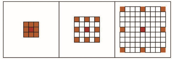
Fig. 1. Dilated convolution

Download full size

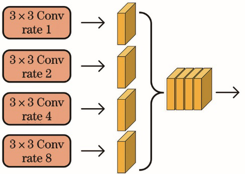
Fig. 2. Parallel multi-branch structure

Download full size

Fig. 3. Attention residual block

Download full size

Fig. 4. Spatial pyramid pooling module

Download full size

Fig. 5. Detailed design of segmentation head in booster

Download full size

Fig. 6. Multi-scale attention analytic network

Download full size

Fig. 7. Training samples and labels. (a) Training samples; (b) labels

Download full size

Fig. 8. Image preprocessing. (a) Original image; (b) preprocessed image

Download full size

Fig. 9. Retinal vessel segmentation results of different algorithms. (a) Original images; (b) labels; (c) results of proposed algorithm; (d) results in Ref. [30]; (e) results in Ref. [17]; (f) results in Ref. [16]; (g) results in Ref. [31]

Download full size

Fig. 10. Detail comparison of segmentation results. (a) Original images; (b) details of original images; (c) details of labels; (d) segmentation details of proposed algorithm; (e) segmentation details of algorithm in Ref. [30]; (f) segmentation details of proposed algorithm in Ref. [17]

Download full size

Fig. 11. ROC curves of segmentation results of different algorithms. (a) ROC curves; (b) curves in box of Fig. 11(a)

Download full size

Fig. 12. PR curves of segmentation results of different algorithms. (a) PR curves; (b) curves in rectangular of Fig. 12(a)

Download full size

Fig. 13. Changes in various evaluation indicators. (a) F₁ value; (b) accuracy; (c) sensitivity; (d) specificity; (e) AUC (ROC); (f) AUC (PR)

Download full size

α	Evaluation Metrics
α	F₁	A	S	S'	AUC (ROC)	AUC (PR)
--	0.8267	0.9669	0.7868	0.9870	0.9858	0.9157
0.6	0.8281	0.9669	0.7940	0.9862	0.9858	0.9158
0.7	0.8301	0.9669	0.8054	0.9849	0.9859	0.9157
0.8	0.8321	0.9669	0.8182	0.9835	0.9857	0.9152
0.9	0.8326	0.9663	0.8351	0.9810	0.9861	0.9155

Table 1. Evaluation metrics for cases not using α values and using different α values

Dataset	Method	F₁	A	S	S'	AUC (ROC)	AUC (PR)
CHASEDB1	SegNet^[30]	0.8083	0.9636	0.7646	0.9858	0.9819	0.8972
	U-Net^[17]	0.7894	0.9600	0.7463	0.9839	0.9773	0.8774
	Attention-UNet^[16]	0.8025	0.9624	0.7619	0.9847	0.9801	0.8898
	FD-UNet^[31]	0.8097	0.9636	0.7728	0.9848	0.9830	0.8991
	MAPNet (ours)	0.8326	0.9663	0.8351	0.9810	0.9861	0.9155
STARE	SegNet^[30]	0.8052	0.9639	0.7598	0.9870	0.9823	0.9082
	U-Net^[17]	0.7935	0.9611	0.7475	0.9851	0.9778	0.8911
	Attention-UNet^[16]	0.8039	0.9632	0.7651	0.9857	0.9804	0.9018
	FD-UNet^[31]	0.8080	0.9641	0.7697	0.9861	0.9826	0.9074
	MAPNet (ours)	0.8256	0.9658	0.8120	0.9832	0.9838	0.9172

Table 2. Average performance evaluation results on CHASEDB1 and STARE

Method	Year	F₁	A	S	S'	AUC
Method in Ref. [32]	2016	--	0.9581	0.7507	0.9793	0.9716
Method in Ref. [27]	2017	0.7332	--	0.7277	0.9712	0.9524
Residual U-Net^[33]	2018	0.7800	0.9553	0.7726	0.9820	0.9779
Recurrent U-Net^[33]	2018	0.7810	0.9622	0.7459	0.9836	0.9803
R2U-Net^[33]	2018	0.7928	0.9634	0.7756	0.9712	0.9815
LadderNet^[15]	2018	0.8031	0.9656	0.7978	0.9818	0.9839
DEU-Net^[13]	2019	0.8037	0.9661	0.8074	0.9821	0.9812
Vessel-Net^[12]	2019	--	0.9661	0.8132	0.9814	0.9860
DFA-Net^[34]	2020	0.8087	0.9679	0.8066	0.9823	0.9839
MAPNet (ours)	2020	0.8326	0.9663	0.8351	0.9810	0.9861

Table 3. Comparison of the method proposed on CHASEDB1 with other advanced methods

Method	Year	F₁	A	S	S'	AUC
Method in Ref. [3]	2012	--	0.9534	0.7548	0.9763	0.9768
Method in Ref. [32]	2016	--	0.9628	0.7726	0.9844	0.9879
Method in Ref. [27]	2017	0.7644	--	0.7680	0.9738	--
Method in Ref. [35]	2019	--	0.9638	0.7735	0.9857	0.9833
Method in Ref. [36]	2019	--	0.9640	0.7523	0.9885	--
Method in Ref. [10]	2020	--	0.9656	0.8068	0.9838	0.9812
MAPNet (ours)	2020	0.8256	0.9658	0.8120	0.9832	0.9838

Table 4. Comparison of proposed method with other advanced methods on STARE

Model	F₁	A	S	S'	AUC (ROC)	AUC (PR)
SubNet_1	0.8158	0.9651	0.7707	0.9868	0.9816	0.9009
SubNet_2	0.8200	0.9657	0.7783	0.9866	0.9832	0.9054
SubNet_3	0.8229	0.9663	0.7813	0.9869	0.9839	0.9085
SubNet_4	0.8228	0.9662	0.7824	0.9867	0.9842	0.9092
SubNet_5	0.8253	0.9666	0.7854	0.9869	0.9846	0.9106
SubNet_6	0.8239	0.9664	0.7832	0.9868	0.9854	0.9132
MAPNet	0.8326	0.9663	0.8351	0.9810	0.9861	0.9155

Table 5. Influence of each module on whole model

Wenjie Luo, Guoqing Han, Xuedong Tian. Retinal Vessel Segmentation Method Based on Multi-Scale Attention Analytic Network[J]. Laser & Optoelectronics Progress, 2021, 58(20): 2017001

Download Citation

Set citation alerts for the article

Tools

Set citation alerts for the article

Save the article for my favorites

Paper Information