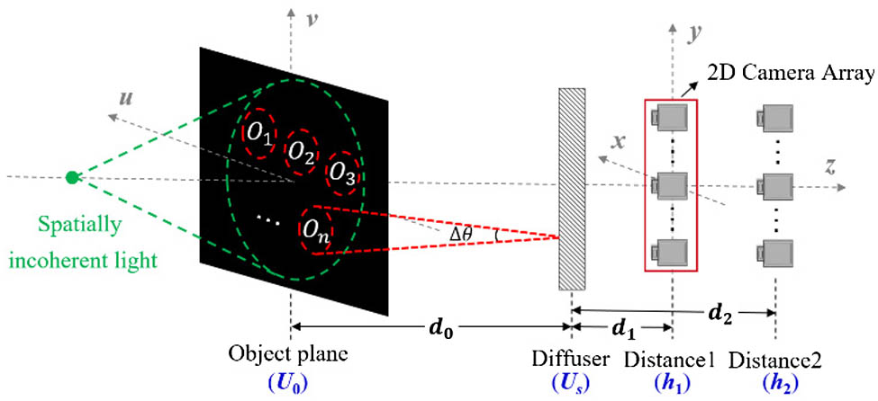
Fig. 1. Schematic of our multi-target large FOV scattering imaging system via the blind target position detection. Multiple isolated targets, O1,O2,…,On, behind the diffuser form a large FOV scene.

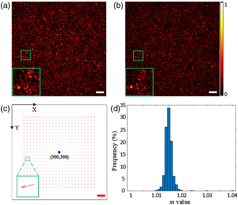
Fig. 2. Simulated experiments to analyze the relationship between two PSFs at different imaging distances (d0=120  mm, pixel size=4.8  μm, 600×600 pixels). The point light source was set at the optical axis (u=300,v=300), as the corresponding point where Ok located in the object plane. (a) Normalized PSFd1k with d1=17  mm. (b) Normalized PSFd2k with d2=19  mm. (c) The estimated low-density scaling vectors based on (a) and (b). The space between any two vectors vertically or horizontally is 20 pixels. The green rectangle in (b) is the matched block of the green rectangle in (a) and the enlarged arrow in (c) represents the estimated scaling vector corresponding to these two green rectangles. The blue point in (c) is the location of the light source. (d) The histogram distribution of m values extracted from all the scaling vectors in (c). Scale bar, 50 camera pixels.

Fig. 3. The block diagram of the scaling-vector-based detection algorithm.

Fig. 4. Multi-target large FOV scattering imaging system setup via the blind target position detection.

Fig. 5. Tests on a real scattering imaging system. (a) The multi-target mask “2FL” with the detailed parameters as the imaging targets. (b) The final large FOV reconstruction with the detected position information. (c) The captured near-field speckle with d2=17.0  mm. (d) The captured near-field speckle with d1=16.5  mm and the extracted autocorrelation of each imaging target centered by the detected locations in (e). (e) The estimated scaling vectors (shown as the red arrows) by block matching and the detected locations (shown as the blue points). The connected component analysis result is shown in the bottom right in a smaller scale. (f)–(j) As in (a)–(e) for a larger and more complex scene “01234.” Scale bar, 50 camera pixels.

Fig. 6. Real tests for biological scattering observation. (a) The neuron-shape mask with the detailed parameters as the imaging targets. (b) The final reconstructed scene. (c) The captured near-field speckle with d1=16.5  mm. Scale bar, 50 camera pixels.

Fig. 7. Real reconstructions for mask “2FL” when the spacing is decreasing from 3.25 mm to 1.5 mm. (a) The original imaging targets with detailed distance parameters. (b) The final reconstructed large FOV scenes corresponding to (a). (c) The averaged PSNRs curve between reconstructions and original targets with respect to the decreasing spacing. (d) The estimated scaling vectors and locations when spacing equals 2.75 mm as an example of reconstructions in good quality. (e) The estimated scaling vectors and locations when spacing equals 1.75 mm as an example of degraded reconstructions.

Table 1. PSNRs Between Reconstructions and Targets