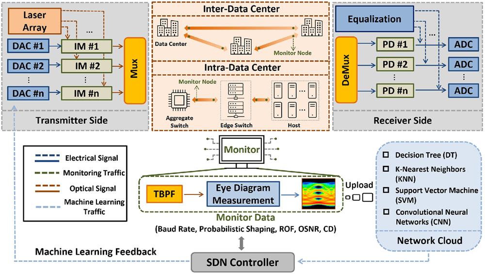
Fig. 1. Conceptual diagram of multiparameter performance monitoring of PAM signals in intra- and inter-data center systems. DAC, digital-to-analog converter; IM, intensity modulator; PD, photodiode; ADC, analog-to-digital converter; TBPF, tunable bandpass filter; SDN, software-defined networking; ROF, roll-off factor; OSNR, optical signal-to-noise ratio; CD, chromatic dispersion.

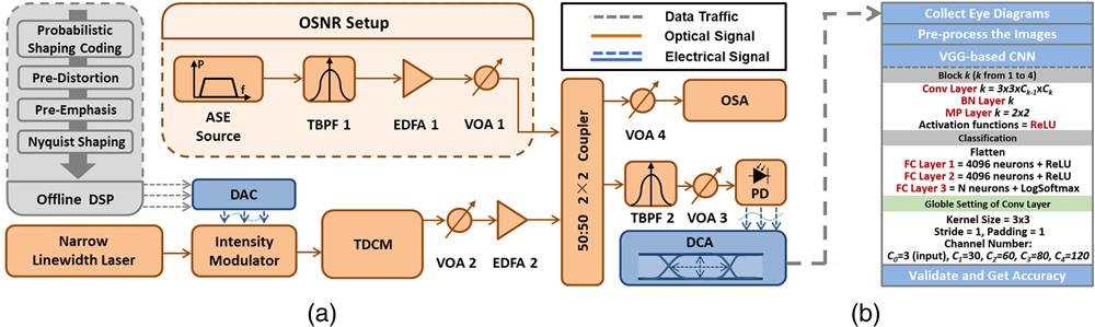
Fig. 2. (a) Experimental setup used to collect eye diagrams. ASE, amplified spontaneous emission; TBPF, tunable bandpass filter; EDFA, erbium-doped fiber amplifier; VOA, variable optical attenuator; DSP, digital signal processing; DAC, digital-to-analog converter; TDCM, tunable dispersion compensation module; PD, photodiode; OSA, optical spectrum analyzer; DCA, digital communication analyzer. (b) The structure of the VGG-based CNN model for classification. Conv, convolutional; BN, batch normalization; MP, max pooling; FC, fully connected.

Fig. 3. Eye diagrams of PAM signals with different MFs, BRs, PS, ROFs, OSNR, and CD.

Fig. 4. Features and parameters used in traditional ML methods (KNN, SVM, DT, and GBDT).

Fig. 5. Typical algorithm architectures applied in the VGG-based model, ResNet-18, MobileNetV3, and EfficientNetV2. PW, point-wise; DW, depth-wise.

Fig. 6. Confusion matrices of DT and GBDT for OSNR, CD, ROF, and BR classification tasks.

Fig. 7. Accuracy of joint monitoring parameters with different ML methods for (a) digital signal parameters and (b) optical link parameters. (c) Accuracy for all the 432 classes for each MF with different five-parameter combinations.

Fig. 8. Accuracy for all 1728 classes with different six-parameter combinations using DT, GBDT, KNN, SVM, and VGG-based CNN.

Fig. 9. (a) Accuracy curves and (b) distributions of VGG-based model, ResNet-18, MobileNetV3-S, and EfficientNetV2-S.

Fig. 10. Structure of MTL model combined with MobileNetV3-Small.

Fig. 11. Accuracy of different monitoring tasks using MTL and VGG-based CNN.

Table 1. Parameters used in hog and color histograms.

Table 2. Structure of the VGG-based model.

Table 3. Accuracy of single-parameter classifications of different ML methods.

Table 4. Parameters selected of traditional ML methods.

Table 5. Accuracy of classifications of GBDT, VGG-based CNN, and VGG-based CNN + GBDT.

Table 6. Computational cost per image of the modern CNN models.

Table 7. Structure of MobileNetV3-Small.

Table 8. Weight of the tasks in the loss function.