There is an extremely complex coercive relationship between urbanization and the eco-environment. Coordinating the relationship between them is a global strategic issue. To address this scientific difficulty, since 2005, a series of international scientific organizations and research programs have carried out research on the topic. In 2005, the International Human Dimensions Program on Global Environmental Change (IHDP) formulated an “urbanization and global environmental change” research plan, which became its core area of work. It proposed strengthening research on the coupling relationship between urbanization and global environmental change using intersecting spatio-temporal scales, spatio-temporal scale comparisons and exchanges between public and policymakers (Jager, 2003). The Millennium Ecosystem Assessment (MEA) report titled “Ecosystems and Human Well-Being” published by the United Nations in 2005 stated that urban populations and economic development will place greater pressure on ecosystems worldwide (MEA, 2005). The theme of the Future Earth project announced in 2012 is to understand the relationship between global environmental change and human well-being and development. This includes cutting-edge research areas such as thresholds, risks and critical points of urbanization, which is the most intense human activity on Earth's surface (Future Earth, 2013). In November 2014, the Science and Technology Alliance for Global Sustainability published Future Earth 2025 Vision, which proposed strengthening eight areas of Future Earth research, including the important area of “urbanization construction” (Fang and Bao, 2008; Fang et al., 2016). On October, 26, 2017, two world-leading international scientific organizations, the International Council for Science (ICSU) and the International Social Science Council (ISSC), convened a conference in Taipei, China, where over 90% of members who voted to merge the two scientific organizations to form the new International Science Council (ISC), which will promote the development of science across disciplines and regions.^*(^* Members of the International Council for Science (ICSU) and International Social Science Council (ISSC) voted in favor of a merger. www.wcsl.org.cn/ind... - 2018-07-28) The establishment and implementation of these major international scientific research programs has pushed the coupling of the natural and social sciences to a new stage of development. It is evident that research on the theories and methods of urbanization and eco-environment coupling will be an important frontier of earth system science research in the coming decade. The current research focus in academia, however, tends to be applied research on urban development as well as evaluations of urban eco-environments and the stability of urban ecosystems. Few studies are on coupling or consist of principle-based research on the organic coupling of the urbanization process and eco-environmental responses. As such, this study starts by looking at the coupling characteristics of interactions between urbanization and the eco-environment and focuses on revealing the coupling relationship and interactive coupling methods in order to develop an urbanization and eco-environment coupling circle theory, produce a “coupling tower” and coupling graphs, and develop a coupler regulation method.

The mutual coupling process between urbanization and the eco-environment is a huge complex system involving social, economic, and natural elements. Scholars from various disciplines have proposed coupling analysis frameworks for this huge system (Chen et al., 2001). These include human and natural system coupling (Liu et al., 2007), “telecoupling,” (Liu et al., 2013) a sustainable livelihood framework (Sherbinin et al., 2008), population, development and environment research frameworks (Dietz et al., 2017; Hummel et al., 2017), social-ecological systems (Ostrom, 2001), planetary boundaries (Steffen, 2015), a DPSIR framework (Tscherning, 2012), a STIRPAT framework and an emergy (embodied energy) analysis framework. In the 21st century, Gunderson has proposed a well-known adaptive nested model of cross-scale systems (Gunderson, 2001). Dietz et al. (2003) have expounded the characteristics of cross-boundary coupling between man and nature. Folke (2006) discussed an elastic method of studying social-ecological systems. And, based on “telecoupling,” Liu (2017) proposed “metacoupling”. These coupling analysis frameworks have provided inspiration for this study. 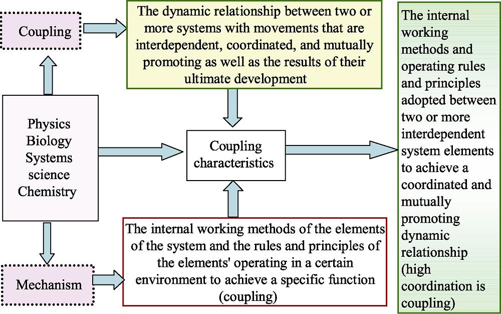The relationship between urbanization and the eco-environment is essentially the relationship between humans and nature, which is reflected in coupling characteristics including coupling intensity, the coupling constant and the coupling agent. Coupling can be characterized as strong or weak, with six levels (very low, low, medium, high, very high and full) of intensity, which correspond to the categories of random coupling, indirect coupling, loose coupling, cooperative coupling, close coupling, and controlled coupling. Together, these make up an urbanization and eco-environment “coupling tower.”

Coupling is a concept commonly used in physics, biology, systems science, and chemistry. It refers to the dynamic relationship between two or more systems with movements that are interdependent, coordinated and mutually promoting, as well as to the result of their ultimate development. Coupling is the internal working methods and operating rules and principles (or technical paths) used by two or more interdependent system elements to achieve a coordinated and mutually promoting dynamic relationship (high coordination is coupling) (Figure 1). Energy transfers and material exchanges between humans and the environment depend on the Earth's surface, and the process of coupling occurs via the atmosphere, hydrosphere, lithosphere, biosphere and noosphere. Coupling characteristics are reflected by the coupling constant, coupling agent and coupling intensity.

Of these, the coupling constant is a critical parameter that indicates that recurrence between the two systems is in a highly cooperative state. Above or below this parameter, coupling between the two systems is broken and they enter a non- cooperative, uncoupled state. At certain time and space scales, the coupling constant is a constant quantity, but the coupling constant changes with changes in time and space in order to find a new coupling constant in the spatio-temporal scale. The coupling agent - also called the coupling medium - refers to media such as materials, energy and information in the exchange process that systems rely on to achieve a certain intensity of coupling. Without the transmission and exchange of material, energy or information between systems, the system is unable to complete the coupling process.

Coupling intensity is a measure of the degree of association and coordination between systems. The greater the connection between systems, the greater the intensity of coupling (indicating that the extent of the connection and of dependence between the systems is close), and the stronger the coupling characteristics. In fact, changes to mutual coercion and coupling between urbanization and the eco-environment are a nonlinear process (Li and Ding, 2004; Qiao and Fang, 2005), and the general functions of changes to coupling areas are as follows:

where x and y are elements of the two systems; a and b are the weights of the elements; and f (U) and f (E) represent the function expressions of the evolution of the urbanization area and the eco-environment area, respectively. They are the leading part of the coupling system according to general systems theory. The equations of the evolution of the coupled system can be expressed as follows:

where A and B are the evolutionary states of the urbanization area and the eco-environment area under the influence of near-distance factors, and V_A and V_B are the evolution speeds of the two areas under the influence of near-distance factors. The evolution speed V of the coupling system composed of the urbanization area and the eco-environment area can be regarded as a function of V_A and V_B (Xu et al., 2003). As such, V = f (V_A, V_B), and because the change of V is caused by V_A and V_B, the evolution trajectories of V_A and V_B can be projected onto a two-dimensional plane (V_A, V_B) to form an ellipse (Figure 2). It can be seen from the figure that angle a between V and V_B is the coupling intensity between the urbanization area and the eco-environment area. Theoretically, in a period of evolution, the coupling system formed by the urbanization area and the eco-environment area will experience four development stages: low-level coordinated development (I, -90°<a≤0°), slow coordinated development (II, 0°<a≤90°), high-speed development (III, 90°<a≤180°) and a rising spiral (IV, -180°<a≤-90°) (Qiao and Fang, 2006).

Based on the intensity of coupling between the urbanization area and the eco-environment area, coupling can be divided into six types: random coupling, indirect coupling, loose coupling, cooperative coupling, close coupling and controlled coupling, which together make up a “coupling tower” between urbanization and the eco-environment (Figure 3 and Table 1).

(1) Random coupling. Random coupling means that there is no relationship between the two major systems of urbanization and the eco- environment, or that the two major systems are independent of each other and do not interfere with each other. The two major systems can cooperate if they wish, or not, but it does not affect the normal function of the systems. Under random coupling, the urbanization system and the eco-environment system have the strongest independence, the lowest degree of coupling, and the weakest, or no correlation. The coupling path is usually an adaptive path, and the strength of coupling is very low. It is the lowest part of the coupling tower.

(2) Indirect coupling. Indirect coupling means that there is no direct relationship between the two systems of urbanization and the eco-environment, or the degree of mutual interference between the two systems is very low, and the degree of association between the two systems is low, with only an indirect relationship, rather than a direct relationship. The urbanization system and the eco-environment system are quite strongly independent, and the intensity of coupling is low, generally between 10% and 30%. The coupling path is usually an adaptive organizational path, and the strength of coupling is low. It has a low position in the coupling tower.

(3) Loose coupling. Loose coupling refers to when one of the two systems of urbanization and the eco-environment accesses another system, exchanges input/output information with each other through data parameters (not control parameters, public data structures or external variables). The loosely coupled urbanization system and the eco-environment system have moderate independence. There is a moderate intensity of coupling, generally between 30% and 50%. The coupling path is usually an adaptive control path, and the strength of coupling is moderate. It has a middle position in the coupling tower.

(4) Cooperative coupling. Cooperative coupling refers to when one of the two systems of urbanization and the eco-environment requires the cooperation of the other system to function normally. The urbanization and eco-environment systems have quite weak independence. The degree of association between them is quite high, and they have quite high coupling intensity, generally between 50% and 70%. The coupling path is usually a regulatory path, and the strength of coupling is high. It occupies an upper-middle position in the coupling tower.

(5) Close coupling. Close coupling refers to a high degree of dependence of one system in the two systems of urbanization and the eco-environment on the other system in order to function normally. The systems have very weak independence. The degree of association between them is quite high, and they have high coupling intensity, generally between 70% and 90%. The coupling path is usually a regulatory path, and the strength of coupling is very high. It occupies a high position in the coupling tower.

(6) Controlled coupling. Within the urbanization and eco-environment systems, controlled coupling is present if a change in the logical relationship of a control parameter within one system affects the normal operation of that system as well as of the other system. Independence of the urbanization system and the eco-environment system is the weakest under controlled coupling. The degree of association between the systems is the highest, and they have very high coupling intensity, generally between 90% and 100%. The coupling path is usually a regulatory path, and the strength of coupling is fully coupled. It sits at the top of the coupling tower.

A complex mutually coercive relationship objectively exists between urbanization and the eco-environment. The future of theoretical research in this area and the question we are trying to answer is which technological path can be used to find the best coupling point of mutual coercion between urbanization and the eco-environment (Fang et al., 2016), so that the urbanization and eco-environment areas of the circle maintain the “best distance” between them and ensure they remain in constant dynamic balance. Urbanization and eco-environment coupling circle theory is based on the theoretical basis of coupling theory, integration theory, combination theory and area theory. It is theoretically supported by a theory on the interaction between regional continuity and development circles from 1999 (Fang, 1999), as well as a theory on mutual coupling between urbanization and the eco-environment, both proposed by authors of this study (Fang and Wang, 2013). Coupling theory and integration theory are one of the ten candidate signs of the sixth scientific and technological revolution (He, 2017).

The urbanization and eco-environment coupling circle theory is based on urbanization and eco-environment mutual coupling theory. It integrates three original areas into two areas, turns original external intervention and regulation into internal self-organization, and changes an original single-line graph into a multi-line graph to create a new theory and new graph. The basic viewpoints of the urbanization and eco-environment coupling circle theory are that a near-distance, nonlinear coupling relationship objectively exists between urbanization and the eco-environment; this nonlinear coupling relationship can be quantified in terms of coupling intensity, and a “coupling tower” can be created based on that intensity; urbanization and eco-environment coupling circles can have linear, exponential-curve, logarithmic-curve, double exponential-curve and S-curve coupling graphs, and the S-curve graph is considered the best graph as it embodies the optimal mutual coupling scenario; coupling circles can be regulated using a developed coupler so that the urbanization and eco-environment areas always remain in the most dynamic and orderly state; over time, the degree of coupling between urbanization and the eco-environment displays a wave-like ascending pattern, which is called the coupling climbing law or coupling ladder, whereby each instance of coupling will rise to a new height, promoting sustainable urban development, and each instance coercion will lead to a decline in sustainable urban development.

In accordance with the urbanization and eco-environment coupling circle theory, to reflect the development stages and urbanization models of different cities, this study has created linear, exponential-curve, logarithmic-curve, double exponential-curve and S-curve coupling graphs of urbanization and eco-environment coupling circles. Each type of graph is divided into nine graphs (Figure 4), which are rotated 10° each time, giving a total of 45 coupling graphs. Different graphs have different principles of change, which correspond to the different development stages, development characteristics and development models of cities.

(1) Urbanization and eco-environment linear coupling graphs. Linear coupling graphs refer to graphs in which the coupling boundary between the urbanization area and the eco-environment area in the course of the evolution of the urbanization and eco-environment coupling circle is in the form of a linear function (Figure 5). The formula is as follows:

where y₀ and x₀ represent the initial contribution of urbanization area and eco-environment area to the coupling circle; y and x represent the final contribution of urbanization area and eco-environment area to the coupling circle; and k represents the coefficient of interactions between the urbanization and eco-environment areas. As the coefficient changes, the contributions of urbanization area U and eco-environment area E to the coupling circle will each increase or decrease, with the areas of the circle changing from eco-environment-dominant (accounting for 100% of the circle), to the eco-environment and urbanization areas each accounting for 50% of the circle, and then to urbanization-dominant (accounting for 100% of the circle). This is an ideal linear coupling model of urbanization and eco-environment evolution, wherein, the driving force on the urbanization area and braking force on the eco-environment area are applied at a uniform speed. This gives coupling circles in which the linear function line is the coupling boundary between the urbanization and eco-environment areas. Urbanization and the eco-environment are two very complex layered systems, so linear urbanization and eco-environment coupling circles do not exist in real life.

(2) Urbanization and eco-environment exponential-curve coupling graphs. Exponential-curve coupling graphs refer to graphs in which the coupling boundary between the urbanization area and the eco-environment area in the course of the evolution of the urbanization and eco-environment coupling circle is in the form of an exponential function (Figure 6). The formula is as follows:

where y₀ and x₀ represent the initial contribution of urbanization area and eco-environment area to the coupling circle; y and x represent the final contribution of urbanization area and eco-environment area to the coupling circle; and k represents the coefficient of interactions between the urbanization and eco-environment areas. As the interaction coefficient changes, the contributions of urbanization area U and eco-environment area E to the coupling circle will each increase or decrease, with the areas of the circle gradually changing from eco-environment-dominant (accounting for 100% of the circle), to the eco-environment and urbanization areas each accounting for 50% of the circle, and then to urbanization-dominant (accounting for 100% of the circle). This is an exponential coupling model of urbanization and eco-environment evolution that objectively exists in reality. It is characterized by accelerated development of urbanization and industrialization and an accelerating driving force to the urbanization area that far exceeds the braking force to the eco-environment area, which causes serious damage to the eco-enviroment. As a result, a coupling circle with the exponential function curve as the coupling boundary between the urbanization and eco-environment areas is formed. A similar exponential curve pattern appears in cities and regions of China in the rapid growth stage of urbanization.

(3) Urbanization and eco-environment logarithmic-curve coupling graphs. Logarithmic-curve coupling graphs refer to graphs in which the coupling boundary between the urbanization area and the eco-environment area in the course of the evolution of the urbanization and eco-environment coupling circle is in the form of a logarithmic function (Figure 7). The formula is as follows:

where y₀ and x₀ represent the initial contribution of urbanization area and eco-environment area to the coupling circle; y and x represent the final contribution of urbanization area and eco-environment area to the coupling circle; and k represents the coefficient of interactions between the urbanization and eco-environment areas. As the interaction coefficient changes, the contributions of urbanization area U and eco-environment area E to the coupling circle will each increase or decrease, with the areas of the circle gradually changing from eco-environment-dominant (accounting for 100% of the circle), to the eco-environment and urbanization areas each accounting for 50% of the circle, and then to urbanization-dominant (accounting for 100% of the circle). This is a logarithmic coupling model of urbanization and eco-environment evolution that objectively exists in reality. It is characterized by accelerated development in the initial stage of urbanization, acceleration of the driving force to the urbanization area, and a gradual weakening of the driving force to the urbanization area in the middle and late stages, but still far exceeding the braking force to the eco-environment area. As a result, a coupling circle with a logarithmic function curve as the coupling boundary between the urbanization and eco-environment areas is formed.

(4) Urbanization and eco-environment double exponential-curve coupling graphs. Double exponential-curve coupling graphs refer to graphs in which the coupling boundary between the urbanization area and the eco-environment area in the course of the evolution of the urbanization and eco-environment coupling circle is in the form of a double exponential function (Figure 8). The double exponential curve is a logical compound of the environmental Kuznets inverted U-curve and logarithmic curve, which reveals that, as urbanization develops, there is a coupling law of exponential decline followed by exponential improvement. The formula is as follows:

where y₀ represents the initial urbanization area of the coupling circle; a, b and c are all non negative parameters; y and x represent the final urbanization area and eco-environment area of the coupling circle; and k represents the coefficient of interactions between the urbanization and eco-environment areas. As the interaction coefficient changes, the contributions of urbanization area U and eco-environment area E to the coupling circle will each increase or decrease, with the areas of the circle gradually changing from eco-environment-dominant (accounting for 100% of the circle), to the eco-environment and urbanization areas each accounting for 50% of the circle, and then to urbanization-dominant (accounting for 100% of the circle). This is a double exponential coupling model of urbanization and eco-environment evolution that objectively exists in reality. It is characterized by accelerated development in the initial stage of urbanization, acceleration of the driving force to the urbanization area, a gradual weakening of the driving force to the urbanization area in the middle and latter stages, a gradual increase in the braking force to the eco-environment area, becoming increasingly restrictive and causing the driving force and direction of force of the urbanization area to change. As a result, a coupling circle with a double exponential function curve as the coupling boundary between the urbanization and eco-environment areas is formed.

(5) Urbanization and eco-environment S-curve coupling graphs. S-curve coupling graphs refer to graphs in which the coupling boundary between the urbanization area and the eco-environment area in the course of the evolution of the urbanization and eco-environment coupling circle is in the form of an S-shaped function (Figure 9). It represents a state of harmony between humans and land (urbanization and the eco-environment) at the start, as the development of the urbanization area takes into consideration protection of the eco-environment, and protection of the eco-environment provides a natural foundation and supports the development of urbanization. As such, it is the optimal coupling graph of urbanization and the eco-environment. The formula is as follows:

where y₀ represents the initial urbanization area of the coupling circle; a, b and c are all non negative parameters; y and x represent the final contribution of urbanization area and eco-environment area to the coupling circle; and k represents the coefficient of interactions between the urbanization and eco-environment areas. As the interaction coefficient changes, the contributions of urbanization area U and eco-environment area E to the coupling circle will each increase or decrease, with the areas of the circle gradually changing from eco-environment-dominant (accounting for 100% of the circle), to the eco-environment and urbanization areas each accounting for 50% of the circle, and then to urbanization-dominant (accounting for 100% of the circle). This is a coupling model of urbanization and eco-environment evolution that objectively exists in reality and conforms with sustainable development goals. It is characterized by accelerated development in the initial stage of urbanization, acceleration of the driving force to the urbanization area, relatively minor braking force on the eco-environment area within a bearable range, a gradual weakening of the driving force to the urbanization area in the middle and late stages, a pattern of mutual fluctuations and checks and balances formed by the braking force of the eco-environment area, and a sustained state of optimum dynamic balance and order between the urbanization area and the eco-environment area. As a result, a coupling circle with an S-shaped function curve as the coupling boundary between the urbanization and eco-environment areas is formed.

A comparative analysis of the linear, exponential-curve, logarithmic-curve, double exponential-curve, and S-curve graphs reveals the following: the linear graph is an ideal graph for coupling urbanization with the eco-environment; the exponential-curve graph is the worst graph for coupling urbanization with the eco-environment; the logarithmic-curve graph is the inferior graph for coupling urbanization with the eco-environment; the double exponential-curve graph is the suboptimal graph for coupling urbanization with the eco-environment; and the S-curve graph is the optimal graph for coupling urbanization with the eco-environment (Figure 10).

By enlarging the optimal S-curve graph to the module level, we can discover the spatial structure of the S-curve graph. Using the S-curve as the coupling boundary, the left half is the urbanization area. It is composed of human elements, such as population, economy, society, and construction land. It is where the main human processes occur based on the laws of humanity (Figure 11). The right half is the eco-environment area, composed of natural elements, such as ecology, environment, pollution, energy, and cultivated land, which follow the laws of nature. The two areas are wedged into, and integrated with, each other to form an organic whole that is mutually existent, dependent and promotional. Water, as a key element of both the urbanization area and the eco-environment area, is located on the coupling boundary between the two areas, indicating that water plays a decisive role in both their coupling process.

If the optimal S-curve graph is enlarged further from the module level to the variable level, we discover that there are 201 variables that help regulate the S-curve graph (Table 2). The causal feedback linkages between each process are shown in Figure 11. The selection of each variable is based on the contribution to the system, comprehensiveness, scientific nature, relevance and data availability of each variable. The choice is based on the causal feedback relationship between each module and other modules, as well as between internal elements of the module, between variables and between parameters. It can be seen from the figure that there is a complex one-to-one, one-to-many, and many-to-many relationship between the various modules and variables within modules. If any variable changes, it has far-reaching effects and influences the structure, function and regulation of the entire coupler.

Dynamic regulation of urbanization and eco-environment coupling includes three major aspects: static regulation between multiple urbanization areas and eco-environment areas at the same time, dynamic regulation between the same urbanization area and eco-environment area at different times, and dynamic regulation between multiple urbanization areas and eco-environment areas at different times.

(1) Static coupling of multiple cities and multiple elements at the same time. This refers to the complex coupling relationships formed by multiple elements of multiple cities at the same time within an urban agglomeration. At different spatial scales at the same time within the agglomeration, this type of regulation is characterized by optimization of the allocation of various resources, environmental improvements, joint construction and sharing of inter-city infrastructure and public services, cooperation between multiple cities, and rational adjustments to multiple elements within multiple cities, to ultimately achieve static coupling within a fixed time. Over time, the multi-element static coupling is quickly broken, and in the new time period, it either evolves into a new static coupling state or leads to static imbalance, depending on the inter-annual optimization and rational allocation of multiple elements in the two time periods.

(2) Dynamic coupling of multiple cities and multiple elements at different times. This refers to the dynamic coupling relationships formed by multiple elements of multiple cities at different times within an urban agglomeration. At different spatial scales at different times within the urban agglomeration, this type of regulation is characterized by different cities in the agglomeration achieving intergenerational optimized allocation of resources, intergenerational improvements in regional eco-environments, intergenerational coordinated construction and sharing of infrastructure and public services between cities, cooperation between multiple cities, and rational adjustments to multiple elements within multiple cities, to ultimately achieve dynamic coupling of multiple cities at different times. As time passes, multi-element dynamic coupling is gradually optimized into a new dynamic coupling state, which will promote the evolution from low-level coupling to high-level coupling between urbanization and the eco-enviroment within the urban agglomeration.

(3) Dynamic coupling of a single city and multiple elements at different times. This refers to the dynamic coupling relationships formed by multiple elements of an urban agglomeration at different times, or by multiple elements of a specific city in an urban agglomeration at different times. At different spatial scales at different times within the urban agglomeration, this type of regulation is characterized by the agglomeration achieving intergenerational optimized allocation of resources, intergenerational improvements in regional eco-environments, intergenerational coordinated construction and sharing of infrastructure and public services between cities, cooperation between multiple cities, and rational adjustments to multiple elements within multiple cities, to ultimately achieve dynamic coupling at different times. As time passes, multi-element dynamic coupling is gradually optimized into a new dynamic coupling state, which will promote the evolution from low-level coupling to high-level coupling between urbanization and the eco-environment within the urban agglomeration.

(1) It has been objectively identified that there is an extremely complex near-distance coupling relationship between urbanization and the eco-environment. We have shown the coupling nature, coupling relationship, coupling intensity and coupling tower of interactions between urbanization and the eco-environment; summarized 10 relationships and interactions of urbanization and eco-environment coupling based on the main control elements; and divided coupling nature according to intensity into six types, namely, very low, low, medium, high, very high and full coupling, which correspond to the categories of random coupling, indirect coupling, loose coupling, cooperative coupling, close coupling, and controlled coupling, thereby forming a “coupling tower” of urbanization and the eco-environment.

(2) We created an urbanization and eco-environment coupling circle theory and graphs. A total of 45 linear, exponential-curve, logarithmic-curve, double exponential-curve and S-curve graphs were generated based on each 10° of rotation, with the different graphs corresponding to different urban development stages, models and characteristics. Of the various coupling graphs, the S-curve coupling graph is considered optimal, as it reflects the best coupling scenario of interactivity between urbanization and the eco-environment.

(3) We developed an urbanization and eco-environment coupler (UEC) for regulation and control. Using an enlarged S-curve coupling graph, and with the help of an SD model and based on the complex one-to-one, one-to-many, and many-to-many relationships between the variables, we developed the UEC, which is composed of 11 regulating elements and 201 variables, for regulation and control. The coupler includes three spatio-temporal scales: static regulation between multiple urbanization areas and eco-environment areas at the same time, dynamic regulation between the same urbanization area and eco-environment area at different times, and dynamic regulation between multiple urbanization areas and eco-environment areas at different times. The coupler ensures the urbanization and eco-environment areas maintain an optimal dynamic and orderly state. Any change in any of the variables changes the whole, affecting the structure, function and regulation of the entire coupler.

(4) Verifying the coupling theory and coupling regulation through applications is an important area of future research. Due to limitations in its scope, this article simply proposed the basic ideas, graphs and coupler for urbanization and eco-environment coupling circle theory. Using the Beijing-Tianjin-Hebei urban agglomeration as a case study for verification, we developed urbanization and eco-environment coupler software, the results of which are published in a separate study. Future studies could analyze other urban agglomerations in order to discover universal principles and draw further conclusions.

References

[1] General System Theory: Foundation, Development, Applications. Rev. ed. New York: George Beaziller(1987).
[2] . Human-Environment System and the Sustainability(2001).
[3] Drivers of human stress on the environment in the twenty-first century. Annual Review of Environment & Resources, 42, 189-213(2017).
[4] The struggle to govern the commons. Science, 302, 1907-1912(2003).
[5] The interaction theory of the regional continuous circle and the development circle. Studies in Dialectics of Nature, 15, 31-33(1999).
[6] . The Process of Urbanization and Ecological Environment Effect(2008).
[7] International progress and evaluation on interactive coupling effects between urbanization and the eco-environment. Journal of Geographical Sciences, 26, 1081-1116(2016).
[8] A theoretical analysis of interactive coercing effects between urbanization and eco-environment. Chinese Geographical Science, 23, 1-16(2013).
[9] et alTheoretical analysis of interactive coupled effects between urbanization and eco-environment in mega-urban agglomerations. Acta Geographica Sinica, 71, 531-550(2016).
[10] Resilience: The emergence of a perspective for social-ecological systems analyses. Global Environmental Change, 16, 253-267(2006).
[11] Future Earth Initial Design: Report of the Transition Team. Paris: International Council for Science (ICSU)(2013).
[12] . Panarchy: Understanding Transformations in Human and Natural Systems(2001).
[13] The forecast and explanation of new revolution of science and technology. Chinese Science Bulletin, 62, 785-798(2017).
[14] et alInter- and transdisciplinary approaches to population-environment research for sustainability aims: A review and appraisal. Population & Environment, 34, 481-509(2013).
[15] The International Human Dimensions Programme on Global Environmental Change (IHDP). Global Environmental Change, 13, 69-73(2003).
[16] Study of coordinated development model and its application between the economy and resources environment in small town. Systems Engineering: Theory & Practice, 24, 134-139(2004).
[17] . Theory, Methods and Application of Stability(1999).
[18] Integration across a metacoupled world. Ecology and Society, 22, 29-47(2017).
[19] et alFraming sustainability in a telecoupled world. Ecology and Society, 18, 26-44(2013).
[20] et alCoupled human and natural systems. Ambio, 36, 639-649(2007).
[21] . Ecosystems and Human Well-being: Synthesis(2005).
[23] The dynamic coupling model of the harmonious development between urbanization and eco-environment and its application in arid area. Acta Ecologica Sinica, 25, 3003-3009(2005).
[24] The coupling law and its validation of the interaction between urbanization and eco-environment in arid area. Acta Ecologica Sinica, 26, 2183-2190(2006).
[26] et alPlanetary boundaries: Guiding human development on a changing planet. Science, 347, 736-747(2015).
[27] et alDoes research applying the DPSIR framework support decision making?. Land Use Policy, 29, 102-110(2012).
[28] et alResearch on the path and early warning of sustainable development. Mathematics in Practice and Theory, 33, 31-37(2003).
Set citation alerts for the article
Please enter your email address
© Copyright 2018-2021 | Chinese Laser Press. All Rights Reserved 沪ICP备15018463号-20