
Zexin Feng, Dewen Cheng, Yongtian Wang. Iterative freeform lens design for optical field control[J]. Photonics Research, 2021, 9(9): 1775
- Photonics Research
- Vol. 9, Issue 9, 1775 (2021)
Abstract
1. INTRODUCTION
A beam transformer converts a given incident beam into a prescribed output beam with certain irradiance and phase (or wavefront) distributions [1]. It has various applications, including lithography, material processing, laser or LED projector, optical communications, and light detection and ranging (lidar). Refractive, reflective, and diffractive optical elements can be used for different configurations of beam transformers [1]. Here, we focus on the commonly used refractive or reflective beam transformers, where ray optics are usually used in the design process. The design problem is mainly governed by three types of equations [2]: the energy conservation within a bundle of rays, the ray-tracing equations dominated by Snell’s law in vector form, and the Malus–Dupin theorem that describes the equal optical path lengths (OPLs) between the input and output wavefronts. Moreover, surface continuity should be considered for fabrication issues. Generally, the design problem is very difficult to handle because the output beam to be produced could have arbitrary amplitude and phase distributions without any
Traditional beam transformers are commonly used for the cases in which the input and output beam wavefronts are kept planar and the irradiance distributions are rotationally symmetric. In the 1960s, Frieden [3] and Kreuzer [4] independently introduced a pair of plano-aspherical lens systems for converting a TEM00 Gaussian laser beam into a circular uniform beam while the output wavefront is kept planar. In their methods, the solutions for the aspheric surfaces can be formulated as an integral equation. Rhodes and Shealy [5] derived a set of ordinary differential equations for achieving the same goal. Many later designs can transform the Gaussian laser beam into collimated output beams with Fermi–Dirac, super-Gaussian, super-Lorentzian, and the flattened Lorentzian distributions (see, e.g., Ref. [6]). Doskolovich
Freeform beam transformer designs without rotational symmetries are mostly restricted to paraxial approximations. In a double-mirror system design, Nemoto
Sign up for Photonics Research TOC. Get the latest issue of Photonics Research delivered right to you!Sign up now
Most of the existing methods applicable for nonparaxial cases are devised for planar or spherical beam wavefronts. For these cases, the design problem can be formulated as a nonlinear PDE of the Monge–Ampère (MA) type [14,15]. The mathematical derivation starts with expressing the target plane coordinates as functions of the first freeform surface and its gradient, where the second freeform surface can be eliminated by imposing the OPL constancy condition. The resulting ray-tracing equations are then imported into the energy conservation between the incident and outgoing beam irradiance distributions to obtain the final MA equation, where the surface integrability condition is imposed to ensure a smooth surface. Such a direct determination has the advantage that the design problem can be described by only one equation but at the cost of an extremely complicated and tedious derivation process. Alternatively, collimated beam shaping problems for reflective or refractive designs can be described using OT theories that acquire an integrable ray mapping by finding a solution to a linear programming problem [16–19]. Rubinstein and Wolansky [20] showed that a single lens with two freeform surfaces for shaping arbitrary collimated beams can also be found by solving a variational problem related to the weighted least action. Oliker
There are very few design methods available for complex input and output wavefronts. Feng
We propose a new iterative wavefront tailoring (IWT)-based method to tackle the freeform lens design problem for producing a prescribed output beam with a complex irradiance distribution and phase profile. A previous IWT method is developed for designing a freeform lens that can generate a prescribed irradiance distribution on a planar or curved target through the intermediate construction of an outgoing wavefront immediately behind the exit freeform surface [29,30]. This method can simplify the formula derivation process and flexibly generate a variety of freeform optical structures with high accuracy. The major contribution of this work consists in how to deal with the difficulties arising from the additional generation of a complex output phase profile, which could realize optical field control using freeform optics in a simple, flexible, and accurate way. The method is described in detail in Section 2. We verify the method’s effectiveness in Section 3, where we design a double freeform lens for generating an output beam with complex irradiance and phase distributions that can produce a different irradiance distribution at a certain distance behind the first output plane. A comparison with the OT ray mapping method is also included in Section 3.
2. METHOD
We consider here the design of a freeform lens with two freeform surfaces performing a one-to-one mapping of the input optical field into a prescribed output optical field, as sketched in Fig. 1. The amplitude and phase distributions of the input beam are denoted by and respectively, where . The amplitude and phase distributions of the output beam are denoted by and , respectively, where . An arbitrary light ray that goes through point at the input plane strikes the first freeform surface at point and then strikes the second freeform surface at point . The output light ray intersects with the output plane at point . The input wavefront located at a given distance from the input plane is described by position vector , and the output wavefront located at a given distance from the output plane is described by position vector . The refractive indices of the medium at the left side of the first freeform surface and the right side of the second freeform surface are denoted by , and the refractive index of the freeform lens is denoted by .
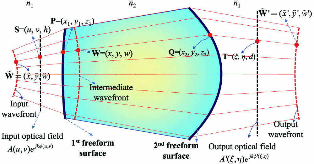
Figure 1.Sketch of the freeform beam transformer.
In the irradiance control IWT method, an outgoing wavefront located behind the exit surface of the freeform lens to be designed is adopted to help solve a ray mapping. For the problem of optical field control, we employ an intermediate wavefront that is next to the entrance freeform surface to be designed. This intermediate wavefront is described by position vector , as illustrated in Fig. 1. In the following, we will first establish the parametrized intermediate wavefront equation, and then describe the IWT procedure specified for optical field control. For the sake of completeness, we also describe the double-freeform surface reconstruction from a ray mapping.
A. Parametrized Intermediate Wavefront Equation
Since we consider a lossless system, and there is no crossing of rays from the input plane to the target plane, the irradiance distributions on the two planes should satisfy the energy conservation in differential form,
We now describe the light propagation properties inside the lens with the help of the intermediate wavefront . According to Fermat’s principle, the first partial derivatives of with respect to and can be described as
Both and can be thought as functions of the independent variables and , and according to chain’s rule,
Herein, . From Eq. (4), we can express as
We denote the unit outgoing ray vectors as . In the framework of geometrical optics, the phase is equivalent to the rays, and the ray directions are determined by the first partial derivatives of the phase (see, e.g., Refs. [31,32]). Therefore, the relationship between and the output phase is
and can be linked through a collinear relationship,
Herein, means the displacement between and , and means the displacement between and . Inserting Eq. (5) into Eq. (7), we obtain
Generally, , , and also are dependent on and . For a degenerate case in which the output beam wavefront is planar, both and are zeros, and the difficulty mainly lies in handling . Such a problem is similar to the irradiance control problem on a curved target where the -values are not constant [30]. Here, we focus on a more complicated case where the output phase is difficult to be expressed analytically. In such a case, and , which are directly relevant with the phase gradient, are difficult to be expressed explicitly with and .
Our solution for simplifying the complicated optical field control problem is to retain and on the right side of Eq. (8) and consider them as functions of the independent variables of and . Equation (8) and its differentiation with respect to and are inserted into Eq. (1) to eliminate the two variables and . The resulting equation is a second-order PDE of MA type,
B. IWT Procedure for Optical Field Control
The IWT procedure for optical field control is illustrated in Fig. 2, and its detailed description is included as follows.
![]()
Figure 2.Diagram of the IWT method for optical field control.
Step 0: We first define an input ray sequence described by the unit input ray vector and an input wavefront from the given input beam information. To start the iterative process, we need to provide an initial estimate of the ray mapping, .
Step 1: From the ray mapping, we acquire the corresponding data of the first partial derivatives of the output phase, and . Then, we immediately determine an output ray sequence according to Eq. (6). From the output ray sequence, we can reconstruct an output wavefront based on least squares, where we employ a concise relationship between the wavefront points and the outgoing ray vectors [27],
Equation (11) means that the chord linking the adjacent wavefront points is perpendicular to the average of the outgoing vectors through the two points. Equation (11) can be written as a linear system of equations of the distances between and , which can be solved with least squares based on Hermann’s method [33] and the MATLAB backslash operator [34].
Step 2: Since we have determined the input ray sequence and wavefront, and the output ray sequence and wavefront, we can compute the double freeform surfaces and to realize the desired transformation using least squares based on Snell’s law and the condition of the OPL constancy [27]. More details are included in Subsection 2.C.
Step 3: After obtaining the data of the double freeform surfaces, we can determine and . We can also obtain an intermediate ray sequence , from which we reconstruct an intermediate wavefront using least squares. Herein, is used to differentiate from in Eq. (9).
Step 4: We insert the data of , and into Eq. (9) and Eq. (10). Taking as the initial value, we solve the MA equation numerically. After obtaining a solution , we can acquire a new ray mapping, , based on Eq. (8).
Step 5: The new ray mapping is inserted into Step 1 to repeat the loop. The stop criterion can be chosen as the difference between the current ray mapping and the previous one or a certain number of iterations.
Step 6: After obtaining the satisfied ray mapping, we need to specify its corresponding output ray sequence and wavefront as in Step 1 and reconstruct the final double freeform surfaces as in Step 2.
Such an iterative procedure can make the freeform lens design for complicated optical field control easier to implement. Although a sequence of MA equations needs to be solved, a multiscale strategy [29,30] for the irradiance control IWT methods can be adapted to speed up the computation here.
C. Double Freeform Surface Reconstruction from the Ray Mapping
Here, we recall the reconstruction of double freeform surfaces following the one-to-one mapping between an input ray sequence and an output ray sequence using a least squares-based iterative procedure [27], which is effective and fast. The basic steps are as follows.
Step 0: We first give an initial approximation of the entrance freeform surface, which can be simply set as a plane.
Step 1: After that, we can obtain a corresponding exit freeform surface based on the constant OPL condition,
Step 2: The required unit ray sequence inside the lens can be acquired as . After that, the required normal field of the first freeform surface can be acquired based on Snell’s law in vector form, .
Step 3: Notice that the normal field is not necessarily integrable and there generally does not exist an exact freeform surface that is perpendicular to everywhere. Therefore, we also employ a least squares method to compute an approximate freeform surface , and the basic relationship between and is [27]
Equation (13) can be written as a linear system of equations of the distances between and , which can also be solved using Hermann’s method and the MATLAB backslash operator.
Step 4: The updated entrance freeform surface is inserted into Step 1 to obtain a new exit freeform surface . The above process is repeated until a required stop criterion is satisfied.
3. RESULTS
As a demonstrative example, we design a freeform lens with the refractive index of 1.5 for transforming a divergent elliptical Gaussian beam into an specified output beam with a complex irradiance distribution and phase profile (see Fig. 3). The input beam is emitted from a point light source located at the original point, and the full width divergence angles for and directions are 12° and 36°, respectively. Figure 3(a) shows the input beam irradiance on the plane, where . The input beam phase distribution , which corresponds to a spherical wavefront, is shown in Fig. 3(b). Figure 3(c) shows the desired output beam irradiance distribution on the plane of , where . Figure 3(d) shows the desired output phase distribution , which is rather irregular and can be difficult to describe by an analytical formula. This phase distribution is aimed for converting into a different irradiance distribution on the plane of [see Fig. 3(e)], where . is obtained by numerically solving a phase-retrieval problem from the two output irradiance distributions [35],
![]()
Figure 3.(a) Irradiance and (b) phase distributions of the input beam on the
The computation size is desired as . To speed up the computation, we employ a multiscale strategy that is similar to that in Refs. [29,30]. The initial computation size is set to . In this step, the initial ray mapping is obtained from solving a standard MA equation corresponding to the OT (see e.g., Ref. [27]),
Let denote the mean absolute deviation of the angles between the computed normals to the entrance freeform surface, i.e., , and the required normals for reconstructing the entrance freeform surface in each IWT iteration. Figure 4 illustrates the effectiveness of the proposed multiscale IWT algorithm in the reduction of the value. The value for the final entrance freeform surface is 0.0064°. Figures 5(a) and 5(b) show the final entrance and exit freeform surfaces, respectively, where you can observe structures that can cause difficulties in analytical expression.
![]()
Figure 4.Evolution of the
![]()
Figure 5.Designed (a) entrance and (b) exit freeform surfaces.
The scattered data points of the double freeform surfaces are inserted into Rhinoceros to create a solid lens model. We implement Monte Carlo ray tracing with rays in LightTools 9.0 to demonstrate the performance of the designed freeform lens. Figure 6(a) visualizes the ray-tracing results of the designed freeform lens in LightTools. Figures 6(b) and 6(c) show the simulated irradiance distributions on the first and second output planes, respectively. It can be seen that the simulated irradiance distribution on the first output plane agrees well with the desired output irradiance distribution shown in Fig. 3(c). The simulated irradiance distribution on the second output plane is also in line with the desired one shown in Fig. 3(e), implying that the output phase on the first output plane is achieved well.
![]()
Figure 6.Simulated results of the freeform lens designed with the new proposed method: (a) ray-tracing illustration in LightTools, and simulated irradiance distributions on the (b) first and (c) second output planes, respectively. Simulated results of the freeform lens designed with the
We provide an OT ray-mapping design for comparison. The OT ray mapping is also calculated in a multiscale way: the computed potential by solving Eq. (15) for a coarser grid is linearly interpolated into an initial value for a finer grid. The double-surface reconstruction following the OT ray mapping is the same as that described in Section 2.C. Since the design geometry is far beyond the paraxial and small-angle approximation, the value for the OT ray-mapping design is as high as 2.3197°, resulting in severe deformations in the simulation results, as shown in Figs. 6(d), 6(e), and 6(f).
We employ the relative root-mean-square deviation (RRMSD) to quantify the deviation of the simulated irradiance distribution from the prescribed one: , where and denote the matrices of the prescribed and simulated irradiance distributions, respectively, within the given domain, and refers to the Frobenius norm [37]. For the OT ray-mapping method, the RRMSD values for the two simulated irradiance distributions can be higher than 0.329. The RRMSD values can be greatly reduced to be lower than 0.045 when we employ the new proposed method.
Figure 7(a) provides the final ray mapping for the new proposed method. Figure 7(b) shows the OT ray mapping. It seems that the two ray mappings demonstrate similar deformations: those regions corresponding to the edges of the numerals are more strongly deformed. However, sufficient differences exist between the two ray mappings, as visualized in Fig. 7(c). The average distance between the two ray mapping is 0.2775 mm. As can be seen from Fig. 7(c), the ray-mapping differences around the central region have relatively small amplitudes, demonstrating that OT ray mapping is more accurate for the paraxial region. However, it does not seem that the central regions on the two simulated irradiance distributions have better performances than the surrounding regions. The holes in the two simulated irradiance distributions of the OT ray-mapping design are caused by a small “bump” around the center of the entrance freeform surface. This small bump is a result of implementing least squares surface reconstruction with a preset value of the center surface point when the normal error is large. We can observe whirls in Fig. 7(c), which may reflect the fact that the OT ray mapping cannot lead to curl-free surface integration. Note that larger errors will occur when we reconstruct the double freeform surfaces according to the OT ray mapping using a point-by-point integration strategy, as described in Ref. [11].
![]()
Figure 7.(a) Final ray mapping of the new proposed method; (b) the
The discrepancies between the new proposed method and the OT ray-mapping method can be narrowed for those designs which satisfy or do not deviate much from paraxial or small-angle approximation. Figure 8 provides a comparison of two freeform lenses designed with the two methods, respectively, for a case that the input beam becomes circular (the full width divergence angles for both and directions are 36°). The RRMSD values for the simulated irradiance distributions of the two freeform lenses become very close. The reason is that the OT ray mapping becomes much closer to the ray mapping computed by the new proposed method. The average distance between the two ray mappings is 0.0275 mm. However, the freeform lens designed with the new proposed method still performs better enough in terms of surface accuracy. The value for the freeform lens designed with the new proposed method is 0.0071°, while the value for the freeform lens designed with the OT ray-mapping method is 0.2119°. The normal error difference between the two lenses can result in larger irradiance discrepancies on receiving planes far away from the lenses.
![]()
Figure 8.Simulated results of the freeform lens designed with the new proposed method: (a) ray-tracing illustration in LightTools, and simulated irradiance distributions on the (b) first and (c) second output planes, respectively. Simulated results of the freeform lens designed with the
4. CONCLUSION
We have proposed a new IWT-based method in designing double freeform optical surfaces for transforming a given optical field into a prescribed one. This method simplifies the design by gradually tailoring an intermediate wavefront next to the entrance freeform surface and incorporating the data of the output phase gradient and the coordinate of the second freeform surface associated with the ray mapping into the IWT procedure. The solution to the wavefront equation leads to a ray mapping between the input beam and the output beam. Approximate first and second freeform surfaces are reconstructed following the ray mapping via an iterative reconstruction procedure based on ray-tracing equations and the constancy of OPLs. The new reconstructed double freeform surfaces can be used to obtain an updated wavefront equation that brings a new ray mapping. Such an iterative process can be implemented in a multiscale way to reduce calculation complexities. Results show that we can obtain a double-freeform lens generating two different irradiance distributions on two successive target planes with much better performances than those of the OT ray mapping method for a case that deviates much from the paraxial or small-angle approximation.
Compared with the previous IWT methods for irradiance control, where a single freeform surface could be enough [29,30], the proposed method can realize additional generation of a prescribed output phase distribution requiring at least double freeform surfaces. This method is also applicable for designing double freeform reflective surfaces or a double plano-freeform lenses system. Such a special iteration strategy may also work with other methods, including the direct determination.
Currently, this method is restricted to those cases in which there are no zero values in the output beam irradiance distributions and there are no extreme local curvatures (or singularities) in the lens surfaces and the input and output wavefronts. We also need to mention that the starting geometry of the lens should be chosen to avoid unphysical solutions.
APPENDIX A
The four coefficients of Eq. (
Herein , , , , , and .
References
[1] D. L. Shealy, F. M. Dickey, J. A. Hoffnagle. Geometrical methods. Laser Beam Shaping: Theory and Techniques, 195-282(2014).
[2] R. Winston, J. C. Miñano, P. Benítez. Nonimaging Optics(2005).
[3] B. R. Frieden. Lossless conversion of a plane laser wave to a plane wave of uniform irradiance. Appl. Opt., 4, 1400-1403(1965).
[4] J. L. Kreuzer. Coherent light optical system yielding an output beam of desired intensity distribution at a desired equiphase surface. U.S. patent(1969).
[5] P. W. Rhodes, D. L. Shealy. Refractive optical systems for irradiance redistribution of collimated radiation: their design and analysis. Appl. Opt., 19, 3545-3553(1980).
[6] D. L. Shealy, J. A. Hoffnagle. Review: design and analysis of plano-aspheric laser beam shapers. Proc. SPIE, 8490, 849003(2012).
[7] L. L. Doskolovich, D. A. Bykov, K. V. Andreeva, N. L. Kazanskiy. Design of an axisymmetrical refractive optical element generating required illuminance distribution and wavefront. J. Opt. Soc. Am. A, 35, 1949-1953(2018).
[8] K. Nemoto, T. Fujii, N. Goto. Laser beam-forming by deformable mirror. Proc. SPIE, 2119, 155-161(1994).
[9] D. L. Shealy, S. H. Chao. Design and analysis of an elliptical Gaussian laser beam shaping system. Proc. SPIE, 4443, 24-35(2001).
[10] Z. Feng, L. Huang, M. Gong, G. Jin. Beam shaping system design using double freeform optical surfaces. Opt. Express, 21, 14728-14735(2013).
[11] Z. Feng, L. Huang, G. Jin, M. Gong. Designing double freeform optical surfaces for controlling both irradiance and wavefront. Opt. Express, 21, 28693-28701(2013).
[12] Z. Feng, B. D. Froese, C. Huang, D. Ma, R. Liang. Creating unconventional geometric beams with large depth of field using double freeform-surface optics. Appl. Opt., 54, 6277-6281(2015).
[13] C. Bösel, H. Gross. Ray mapping approach in double freeform surface design for collimated beam shaping. Proc. SPIE, 9950, 995004(2016).
[14] Y. Zhang, R. Wu, P. Liu, Z. Zheng, H. Li, X. Liu. Double freeform surfaces design for laser beam shaping with Monge-Ampère equation method. Opt. Commun., 331, 297-305(2014).
[15] S. Chang, R. Wu, A. Li, Z. Zheng. Design beam shapers with double freeform surfaces to form a desired wavefront with prescribed illumination pattern by solving a Monge-Ampère type equation. J. Opt., 18, 125602(2016).
[16] T. Glimm, V. Oliker. Optical design of two-reflector systems, the Monge-Kantorovich mass transfer problem and Fermat’s principle. Indiana Univ. Math. J., 53, 1255-1278(2004).
[17] V. Oliker. Optical design of freeform two-mirror beam-shaping systems. J. Opt. Soc. Am. A, 24, 3741-3752(2007).
[18] V. Oliker. Designing freeform lenses for intensity and phase control of coherent light with help from geometry and mass transport. Arch. Ration. Mech. Anal., 201, 1013-1045(2011).
[19] T. Glimm, N. Henscheid. “Iterative scheme for solving optimal transportation problems arising in reflector design. ISRN Appl. Math., 2013, 635263(2013).
[20] J. Rubinstein, G. Wolansky. Intensity control with a free-formlens. J. Opt. Soc. Am. A, 24, 463-469(2007).
[21] V. Oliker, L. L. Doskolovich, D. A. Bykov. Beam shaping with a plano-freeform lens pair. Opt. Express, 26, 19406-19419(2018).
[22] A. Mingazov, D. Bykov, E. Bezus, L. Doskolovich. On the use of the supporting quadric method in the problem of designing double freeform surfaces for collimated beam shaping. Opt. Express, 28, 22642-22657(2020).
[23] L. L. Doskolovich, D. A. Bykov, E. S. Andreev, E. A. Bezus, V. Oliker. Designing double freeform surfaces for collimated beam shaping with optimal mass transportation and linear assignment problems. Opt. Express, 26, 24602-24613(2018).
[24] N. K. Yadav, J. H. M. ten Thije Boonkkamp, W. L. Ijzerman. Computation of double freeform optical surfaces using a Monge–Ampère solver: application to beam shaping. Opt. Commun., 439, 251-259(2019).
[25] S. Wei, Z. Zhu, Z. Fan, Y. Yan, D. Ma. Double freeform surfaces design for beam shaping with non-planar wavefront using an integrable ray mapping method. Opt. Express, 27, 26757-26771(2019).
[26] K. Desnijder, P. Hanselaer, Y. Meuret. Ray mapping method for off-axis and non-paraxial freeform illumination lens design. Opt. Lett., 44, 771-774(2019).
[27] Z. Feng, B. D. Froese, R. Liang, D. Cheng, Y. Wang. Simplified freeform optics design for complicated laser beam shaping. Appl. Opt., 56, 9308-9314(2017).
[28] C. Bösel, H. Gross. Double freeform illumination design for prescribed wavefronts and irradiances. J. Opt. Soc. Am. A, 35, 236-243(2018).
[29] Z. Feng, D. Cheng, Y. Wang. Iterative wavefront tailoring to simplify freeform optical design for prescribed irradiance. Opt. Lett., 44, 2274-2277(2019).
[30] Z. Feng, D. Cheng, Y. Wang. Iterative freeform lens design for prescribed irradiance on curved target. Opto-Electron. Adv., 3, 200010(2020).
[31] L. L. Doskolovich, N. L. Kazanskiy, V. A. Soifer, S. I. Kharitonov, P. Perlo. A DOE to form a line-shaped directivity diagram. J. Mod. Opt., 51, 1999-2005(2004).
[32] J. Rubinstein, G. Wolansky, Y. Weinberg. Ray mappings and the weighted least action principle. J. Math. Industry, 8, 6(2018).
[33] J. Hermann. Least-squares wave front errors of minimum norm. J. Opt. Soc. Am., 70, 28-35(1980).
[35] Z. Feng, D. Cheng, Y. Wang. Transferring freeform lens design into phase retrieval through intermediate irradiance transport. Opt. Lett., 44, 5501-5504(2019).
[36] http://www.siam.org/books/fa01/. http://www.siam.org/books/fa01/

Set citation alerts for the article
Please enter your email address
© Copyright 2018-2021 | Chinese Laser Press. All Rights Reserved 沪ICP备15018463号-20