Quantum-limited resolution of partially coherent sources

Ben Wang; Liang Xu; Hongkuan Xia; Aonan Zhang; Kaimin Zheng; Lijian Zhang

doi:10.3788/COL202321.042601

Abstract

Discriminating two spatially separated sources is one of the most fundamental problems in imaging. Recent research based on quantum parameter estimation theory shows that the resolution limit of two incoherent point sources given by Rayleigh can be broken. However, in realistic optical systems, there often exists coherence in the imaging light field, and there have been efforts to analyze the optical resolution in the presence of partial coherence. Nevertheless, how the degree of coherence between two point sources affects the resolution has not been fully understood. Here, we analyze the quantum-limited resolution of two partially coherent point sources by explicitly relating the state after evolution through the optical systems to the coherence of the sources. In particular, we consider the situation in which coherence varies with the separation. We propose a feasible experiment scheme to realize the nearly optimal measurement, which adaptively chooses the binary spatial-mode demultiplexing measurement and direct imaging. Our results will have wide applications in imaging involving coherence of light.

Keywords

partial coherence quantum imaging quantum metrology

1. Introduction

Imaging is one of the most important applications in optics, ranging from microscopy to astronomy. Achieving higher resolution is the main task in the imaging problem, while the conventional imaging system is limited to the diffraction of light, which is defined by Rayleigh^[1] and known as the Rayleigh criterion. The Rayleigh criterion indicates that two incoherent point sources are regarded as just resolved when the maximum of the illuminance produced by one point coincides with the first minimum of the illuminance produced by the other point. Many theoretical works and technical methods have been proposed to improve the imaging resolution, such as scanning electron microscopy^[2,3] and stimulated emission depletion^[4,5]. These methods aim to get a narrower point spread function (PSF), which do not overcome the Rayleigh resolution limit in principle.

With the development of quantum mechanics and statistics, whether distinguishing two point sources in quantum formulation could beat the Rayleigh resolution limit or not has been re-examined. For this purpose, imaging was cast as a parameter estimation problem^[6–8]. Direct imaging based on intensity measurement leads to infinite uncertainty of separation estimation, as two incoherent point sources are close enough, which is called Rayleigh’s curse^[9], while the fundamental precision limit of the estimation quantified by quantum Fisher information^[10] remains a constant. In the few years since, many other works expanded this problem to more realistic scenarios^[11–21]. The works mentioned above only consider incoherent sources, while imaging an object with coherent light is also an essential problem. It has been shown that the resolution of two coherent point sources depends on the relative phase between them^[22,23], and degree of coherence plays a key role in the resolution^[24,25]. In recent years, two point sources’ resolution with partial coherence provoked wide discussions^[26–28]. It was shown that the existence of coherence will reduce the resolution of two point sources when the separation tends to zero, and Rayleigh’s curse will be resurgent in the completely coherent case^[26]. This conclusion has been extensively debated^[27–29], mainly focusing on the accuracy of the model and how to parameterize the coherence. Ref. [30] points out that the number of total photons detected by measurement devices is changed by the degree of coherence, which is the main controversy in previous works. In this work, we renormalize the quantum state in the imaging plane and model the imaging problem in terms of the coherence of the sources, and this modeling approach gives a clear picture of the effect of the sources’ coherence on the resolution, as well as the change in coherence during the transmission of the optical field. In addition, we also consider the degree of coherence changes with the separation of two sources, which is a ubiquitous effect in practical imaging applications. We will give the optimal measurement method for both cases.

2. Theory

We begin with two partially coherent point sources with the transverse positions $x_{1}$ and $x_{2}$ in the object plane. The initial state $ρ_{ini}$ can be modeled as a probabilistic mixture of incoherent and coherent in-phase components, $ρ_{ini} = \frac{1 - p}{2} (| 1 〉 〈 1 | + | 2 〉 〈 2 |) + \frac{p}{2} (| 1 〉 + | 2 〉) (〈 1 | + 〈 2 |),$ (1)where $| 1 〉 : = \int d x ϕ (x - x_{1}) {\hat{a}}^{†} (x) | 0 〉$ and $| 2 〉 : = \int d x ϕ (x - x_{2}) {\hat{a}}^{†} (x) | 0 〉$ are defined with respect to creation operator ${\hat{a}}^{†}$ . $ϕ (x)$ is the wave function of the photon emitted by source $I_{source} (X)$ and satisfies the normalization condition $\int | ϕ {(x)}^{2} | d x = 1$ . An essential property of $ϕ (x)$ in the source plane is that it has infinitesimal width, especially compared to the separation between two sources, and hence $〈 1 | 2 〉 = \int ϕ^{*} (x - x_{1}) ϕ (x - x_{2}) d x = 0$ . $p$ is the mixing probability^[26] and equals the degree of coherence $g^{(1)} (x_{1} - x_{2})$ . Two point sources will evolve into $| ψ_{1} 〉$ and $| ψ_{2} 〉$ after propagation through the optical system, and $| ψ_{i} 〉 = \int d x ψ (x - x_{i}) {\hat{a}}^{†} (x) | 0 〉 = \exp (- i \hat{P} x_{i}) | ψ 〉, i = 1, 2,$ (2)where $\hat{P}$ , the momentum operator, equals $- i \partial_{x}$ in the $x$ representation. The PSF $ψ (x) = 〈 x | ψ 〉$ is inversion-symmetric [i.e., $ψ (- x) = ψ (x)$ ] in most cases of interest. We define the separation between two sources $s = x_{1} - x_{2}$ and consider two symmetric point sources with the centroid $(x_{1} + x_{2}) / 2 = 0$ . The final state after evolution becomes $ρ_{s} = I_{0} [| ψ_{1} 〉 〈 ψ_{1} | + | ψ_{2} 〉 〈 ψ_{2} | + p (| ψ_{1} 〉 〈 ψ_{2} | + | ψ_{2} 〉 〈 ψ_{1} |)],$ (3)with $I_{0} = 1 / (2 + 2 d p)$ and $d = Re {〈 ψ_{1} | ψ_{2} 〉}$ . $Re {\cdot}$ denotes the real part. Here, we assume the direction of transmission is perpendicular to the image plane, so the two point sources are in-phase with $d = 〈 ψ_{1} | ψ_{2} 〉$ . The full information about the separation can be divided into two parts: the first one is encoded in the wavefront of the light field, while the second one is encoded in the ratio between the number of received photons and that of the photons emitted by a single emitter^[29,30]. However, to access the latter, one needs to calibrate the single emitter, which is difficult in practice, especially when the separation tends to zero. Therefore, Eq. (3) focuses on the first part of the information.

Sign up for Chinese Optics Letters TOC. Get the latest issue of Chinese Optics Letters delivered right to you！Sign up now

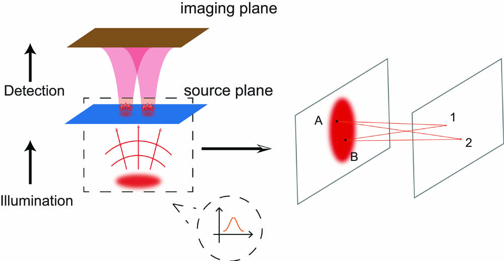
Next, we will consider two cases. (i) The degree of coherence is independent on the separation $s$ between two sources. (ii) The degree of coherence changes with $s$ . An example of the latter case is that the two sources are illuminated by an incoherent source, which is shown in Fig. 1. According to the Van Cittert–Zernike theorem, the relation between the degree of coherence of two point sources, $g^{(1)} (x_{1} - x_{2})$ , in positions $x_{1}$ and $x_{2}$ , and intensity distribution of illumination source can be stated mathematically by $g_{object}^{(1)} (x_{1} - x_{2}) \propto F {I_{source} (X)},$ (4)where $F {\cdot}$ denotes Fourier transformation. If the intensity of incoherent source follows Gaussian distribution, the degree of coherence is also a Gaussian function of spatial separation $p = | g^{(1)} | = \exp (- s^{2})$ .

Figure 1.An example of two point sources with partial coherence. Two point objects are illuminated by an incoherent optical source. Even though the illumination source is completely incoherent, photons arriving at two points in the object plane may share the common origin, which exhibits partial coherence.

To estimate $s$ , we can perform a positive operator-valued measure (POVM) denoted by ${{\hat{M}}_{n}}$ on $ρ_{s}$ , and get the probabilities $p_{n} = tr (ρ_{s} {\hat{M}}_{n})$ , from which we can derive an unbiased parameter estimator $š$ as well as its variance $Δ^{2} s$ . The variance of $N$ trials is bounded by the Cramér–Rao inequality, $Δ^{2} s \geq 1 / (N F_{s})$ ^[10,31,32], with the Fisher information (FI) $F_{s}$ defined by $F_{s} = \sum_{n} \frac{1}{p_{n}} {(\frac{\partial p_{n}}{\partial s})}^{2} .$ (5)

Upon writing $ρ_{s}$ in its eigenbasis, $ρ_{s} = \sum_{n} λ_{n} | e_{n} 〉 〈 e_{n} |$ , quantum Fisher information (QFI) for the parameter $s$ can be calculated by^[12,31] $Q_{s} = 2 \sum_{m n} \frac{{| 〈 e_{m} | \partial_{s} ρ_{s} | e_{n} 〉 |}^{2}}{λ_{m} + λ_{n}},$ (6)where $\partial_{s} ρ_{s} = \partial ρ_{s} / \partial s$ . We have $Q_{s} \geq F_{s}$ , and the equality holds for the optimal measurement^[10]. To determine the QFI of the quantum state in Eq. (3) with respect to parameter $s$ , we decompose the density matrix defined by Eq. (3) in terms of its eigenbasis, $| e_{1} 〉 = \frac{1}{\sqrt{2 (1 - d)}} (| ψ_{1} 〉 - | ψ_{2} 〉), | e_{2} 〉 = \frac{1}{\sqrt{2 (1 + d)}} (| ψ_{1} 〉 + | ψ_{2} 〉),$ (7)and $λ_{1} = (1 - p) (1 - d) I_{0}, λ_{2} = (1 + p) (1 + d) I_{0} .$ (8)

Furthermore, the quantum state defined by Eq. (3) is rank-2. Therefore the QFI can be reduced to a simpler form^[12], $Q_{s} = - \frac{3}{λ_{1}} {| 〈 e_{1} | \partial_{s} ρ_{s} | e_{1} 〉 |}^{2} - \frac{3}{λ_{2}} {| 〈 e_{2} | \partial_{s} ρ_{s} | e_{2} 〉 |}^{2} + 4 (1 - \frac{1}{λ_{1}} - \frac{1}{λ_{2}}) {| 〈 e_{1} | \partial_{s} ρ_{s} | e_{2} 〉 |}^{2} + \frac{4}{λ_{1}} 〈 e_{1} | {(\partial_{s} ρ_{s})}^{2} | e_{1} 〉 + \frac{4}{λ_{2}} 〈 e_{2} | {(\partial_{s} ρ_{s})}^{2} | e_{2} 〉 .$ (9)

By using the condition of the inversion-symmetric PSF, we can get $〈 ψ | {\hat{P}}^{k} | ψ 〉 = 0$ , for any odd $k$ . Therefore, Eq. (9) can be further simplified, $Q_{s} = \frac{{(\partial_{s} λ_{1})}^{2}}{λ_{1}} + \frac{{(\partial_{s} λ_{2})}^{2}}{λ_{2}} + 4 λ_{1} Γ_{1} + 4 λ_{2} Γ_{2},$ (10)where $Γ_{1} = 〈 \partial_{s} e_{1} | \partial_{s} e_{1} 〉$ and $Γ_{2} = 〈 \partial_{s} e_{2} | \partial_{s} e_{2} 〉$ . For this quantum state, the direct imaging that projects the state into the eigenstates of the spatial coordinates $x$ leads to the probability density, $ρ (x) = 〈 x | ρ_{s} | x 〉 = I_{0} [| ψ_{1} (x {) |}^{2} + | ψ_{2} (x {) |}^{2} + 2 p ψ_{1} (x) ψ_{2} (x)] .$ (11)

Because the two point sources are in-phase, we can consider that $ψ_{1} (x)$ and $ψ_{2} (x)$ are real functions. The FI of direct imaging $F_{d}$ is defined by $F_{d} = \int_{- \infty}^{+ \infty} \frac{1}{ρ (x)} {[\frac{\partial ρ (x)}{\partial s}]}^{2} d x$ . To illustrate the results, we consider, for convenience, Gaussian PSF $ψ (x) = {(2 π)}^{- 1 / 4} \exp (- x^{2} / 4)$ with a normalized coordinate with respect to the PSF’s width.

3. Results

For a constant degree of coherence, Fig. 2 shows that QFI varies with the change of the separation $s$ , which has a small difference from Fig. 3 in Ref. [26], mainly due to the parameterization of coherence. We reproduce the results in Ref. [28] in a different way and confirm the validity of that. In the limit $p = 0$ , which corresponds to the incoherent model, QFI is independent of $s$ . While $p = 1$ , which is the totally coherent case, QFI tends to zero when $s$ equals zero, and Rayleigh’s curse is resurgent.

Figure 2.QFI for the estimation of the separation of two partially coherent sources with different degrees of coherence p; the FI of SPADE equals the QFI.

Figure 3.QFI and FI of direct imaging with the intensity measurement F_d for the estimation of the separation of two partially coherent sources with separation-dependent degree of coherence p; even though QFI drops to zero as the separation approaches zero, in the sub-Rayleigh region, where s < 2, QFI is much larger than F_d. QFI and FI meet at large separation.

Spatial-mode demultiplexing (SPADE), which projects the light field into Hermite–Gaussian (HG) spatial modes^[9], is an optimal measurement method for resolving two incoherent point sources. We will demonstrate that it is also optimal when the two sources are partially coherent and the degree of coherence is a constant. Here, we adopt the method in Ref. [17], where displaced Gaussian PSF can be expanded in the HG basis, $| ψ_{1} 〉 = \exp (- \frac{s^{2}}{32}) \sum_{n = 0}^{\infty} \frac{s^{n}}{4^{n} \sqrt{n!}} | ϕ_{n} 〉, | ψ_{2} 〉 = \exp (- \frac{s^{2}}{32}) \sum_{n = 0}^{\infty} \frac{{(- s)}^{n}}{4^{n} \sqrt{n!}} | ϕ_{n} 〉,$ (12)where $| ϕ_{n} 〉 = \int_{- \infty}^{+ \infty} ϕ_{n} (x) | x 〉$ , and $ϕ_{n} (x)$ is the $n$ th order HG spatial mode^[9]. SPADE is described by the POVM ${{\hat{Π}}_{n}}$ , where ${\hat{Π}}_{n} = | ϕ_{n} 〉 〈 ϕ_{n} |$ . The probability distribution is given by $p_{n} = I_{0} \exp (- \frac{s^{2}}{16}) \frac{s^{2 n}}{16^{n} n!} [2 + 2 p {(- 1)}^{n}] .$ (13)The classical FI of SPADE calculated by Eq. (13) equals QFI.

The above analysis just considers the situation that the degree of coherence is a constant. However, the degree of coherence $p$ may change with the separation $s$ in practice. For example, as previously stated, $p = \exp (- s^{2})$ . Next, we consider the precision of different measurement methods. As shown in Fig. 3, the FI of direct imaging $F_{d}$ tends to zero when the separation approaches zero. QFI derivated by Eq. (10) also drops to zero for infinitesimal separation. Rayleigh’s curse cannot be avoided. However, in the sub-Rayleigh region where the separation is smaller than the width of the PSF, i.e., $s < 2$ , the QFI is much larger than $F_{d}$ , which indicates that there exists room to improve the resolution in this region.

Next, we will give the measurement methods for resolving sources with a separation-dependent degree of coherence. As shown in Fig. 3, direct imaging cannot saturate quantum Cramér-Rao bound (QCRB) when $s$ is small. Now we analyze whether SPADE measurement can saturate QCRB. Different from the case with a constant degree of coherence $p$ , the classical FI cannot be calculated analytically with an infinite number of HG modes. Therefore, we consider SPADE with a finite number of modes, which has the POVM ${{\hat{Π}}_{0}, {\hat{Π}}_{1}, {\hat{Π}}_{2},\dots, {\hat{Π}}_{k}, \hat{I} - \sum_{i = 0}^{k} {\hat{Π}}_{i}}$ . When $k = 0$ , the POVM has only two elements, and we call it b-SPADE^[9,33,34]. The FI of SPADE with the different mode number $k$ is shown in Fig. 4. As $k$ increases, more FI can be gained from the SPADE.

Figure 4.FI for SPADE with finite mode number k; even b-SPADE with k = 0 has an FI larger than F_d in the sub-Rayleigh region. b-SPADE performs worse than direct imaging in a large separation region and they are equal to each other at s₁ ≈ 2.47.

Although increasing the number of modes can improve the estimation precision, their difference lies mainly in the region where $s$ is large. Moreover, it is challenging to implement SPADE with large $k$ . On the other hand, direct imaging performs well for large $s$ . Therefore, we propose a measurement method to choose b-SPADE measurement and direct imaging adaptively. $F_{d}$ and FI of b-SPADE meet at $s_{1} \approx 2.47$ , and the choice is based on the comparison between estimation of separation $s_{est}$ and $s_{1}$ .

We show the performance of the method with a numerical simulation. As shown in Fig. 5, the starting point of the process is the prior distribution $p (s)$ , which is a uniform distribution in the interval [0,10]. The probability of the measurement outcome is described by the likelihood function $p (n | s)$ . Once the $j$ th measurement result $n_{j}$ is obtained, the posterior probability $p (s | n_{j}, n_{j - 1},\dots, n_{1})$ is updated by Bayes’s rule, $p (s | n_{j},\dots, n_{1}) = \frac{p (s | n_{j - 1},\dots, n_{1}) p (n_{j} | s, n_{j - 1},\dots, n_{1})}{\int p (s | n_{j - 1},\dots, n_{1}) p (n_{j} | s, n_{j - 1},\dots, n_{1}) d s},$ (14)where the integral is the normalization term. The optimal Bayesian estimator is calculated by $s_{est} = \int s \times p (s | n_{j}, n_{j - 1},\dots, n_{1}) d s,$ (15)which corresponds to the mean value of the parameter over the posterior distribution. The simulation results for different $s$ are shown in Fig. 6.

Figure 5.Protocol of the adaptive measurement method. An initial estimation of the separation s is first obtained by direct imaging. By comparing the estimate s_est and s₁, we can choose the b-SPADE or direct imaging. At each step, the choice of different measurement methods is based on the estimation result calculated by the posterior distribution drawn from the last step. N is the number of cycles.

Figure 6.Simulation results for adaptive measurement method conditioned on N = 1000 detected photons; dashed lines are the FI of direct imaging and b-SPADE, and stars are the simulation results calculated by the inverse of the mean squared error.

4. Discussions and Conclusions

Here we consider the situation in which the degree of coherence between two sources is real. In general, the degree of coherence can be complex^[35]. According to the Van Cittert–Zernike theorem, the phase of the degree of coherence, $φ = \frac{π}{λ z} (r_{2}^{2} - r_{1}^{2}),$ (16)where $λ$ is the wavelength and $z$ is the distance from the incoherent optical source to the object plane, as shown in Fig. 1. In Eq. (16), $r_{1}$ and $r_{2}$ represent, respectively, the distances of the two point sources from the center of the incoherent optical source. The phase factor of degree of coherence can drop if the two conditions can be identified^[36]: (1) if the distance $z$ is much larger than $z ≫ 2 [(r_{2}^{2} - r_{1}^{2}) / λ]$ ; (2) if the two point sources in the source plane have equal distance from the center that $r_{1} = r_{2}$ . In our work, a real degree of coherence is valid under these two conditions. If the center of the two sources is unknown, more than one unknown parameter exists in the wave function, and the degree of coherence is complex; we leave this problem to the future work.

With the development of quantum theory of resolving for two incoherent point sources, quantum-limited resolution of two partially coherent sources has aroused great discussion. There are some controversies in the physical model of this problem^[26–28,30]. In this work, we give a new perspective toward resolving these controversies with a grounded model that explicitly considers the contributions from the coherence of the sources and that is acquired through the propagation. For a constant degree of coherence, quantum limit gives a finite resolution between the two sources, and Rayleigh’s curse is resurgent only in the completely coherent case ( $p = 1$ ). If the degree of coherence depends on the separation as given by the Van Cittert–Zernike theorem, Rayleigh’s curse cannot be avoided. However, in the sub-Rayleigh region where the separation is smaller than the width of PSF, there exists room to improve the resolution compared to direct imaging. SPADE is the optimal measurement method for both cases, while it is challenging to realize experimentally. For a separation-dependent degree of coherence, we propose a feasible measurement method by adaptively choosing direct imaging and binary SPADE, and give the simulation result, which corresponds well to the theory. Our work can also be extended to the more complicated situations in which more unknown parameters such as the centroid and intensity ratio of the two sources are to be estimated.

Note: We are aware of the related independent work in Ref. [37].

References

[1] L. Rayleigh. XXXI. Investigations in optics, with special reference to the spectroscope. Lond. Edinb. Dublin Philos. Mag. J. Sci., 8, 261(1879).

[2] H. J. Leamy. Charge collection scanning electron microscopy. J. Appl. Phys., 53, R51(1982).

[3] D. Drouin, A. R. Couture, D. Joly, X. Tastet, V. Aimez, R. Gauvin. Casino v2.42—a fast and easy-to-use modeling tool for scanning electron microscopy and microanalysis users. Scanning, 29, 92(2007).

[4] T. A. Klar, S. W. Hell. Subdiffraction resolution in far-field fluorescence microscopy. Opt. Lett., 24, 954(1999).

[5] S. W. Hell, J. Wichmann. Breaking the diffraction resolution limit by stimulated emission: stimulated-emission-depletion fluorescence microscopy. Opt. Lett., 19, 780(1994).

[6] C. W. Helstrom. Resolvability of objects from the standpoint of statistical parameter estimation. J. Opt. Soc. Am., 60, 659(1970).

[7] C. W. Helstrom. Quantum Detection and Estimation Theory(1976).

[8] E. Betzig. Proposed method for molecular optical imaging. Opt. Lett., 20, 237(1995).

[9] M. Tsang, R. Nair, X.-M. Lu. Quantum theory of superresolution for two incoherent optical point sources. Phys. Rev. X, 6, 031033(2016).

[10] S. L. Braunstein, C. M. Caves. Statistical distance and the geometry of quantum states. Phys. Rev. Lett., 72, 3439(1994).

[11] F. Yang, R. Nair, M. Tsang, C. Simon, A. I. Lvovsky. Fisher information for far-field linear optical superresolution via homodyne or heterodyne detection in a higher-order local oscillator mode. Phys. Rev. A, 96, 063829(2017).

[12] J. Řehaček, Z. Hradil, B. Stoklasa, M. Paúr, J. Grover, A. Krzic, L. L. Sánchez-Soto. Multiparameter quantum metrology of incoherent point sources: towards realistic superresolution. Phys. Rev. A, 96, 062107(2017).

[13] C. Napoli, S. Piano, R. Leach, G. Adesso, T. Tufarelli. Towards superresolution surface metrology: quantum estimation of angular and axial separations. Phys. Rev. Lett., 122, 140505(2019).

[14] Z. Yu, S. Prasad. Quantum limited superresolution of an incoherent source pair in three dimensions. Phys. Rev. Lett., 121, 180504(2018).

[15] B. Wang, L. Xu, J. C. Li, L. Zhang. Quantum-limited localization and resolution in three dimensions. Photon. Res., 9, 1522(2021).

[16] L. J. Fiderer, T. Tufarelli, S. Piano, G. Adesso. General expressions for the quantum Fisher information matrix with applications to discrete quantum imaging. PRX Quantum, 2, 020308(2021).

[17] E. Bisketzi, D. Branford, A. Datta. Quantum limits of localisation microscopy. New J. Phys., 21, 123032(2019).

[18] J. M. Donohue, V. Ansari, J. Řeháček, Z. Hradil, B. Stoklasa, M. Paúr, L. L. Sánchez-Soto, C. Silberhorn. Quantum-limited time-frequency estimation through mode-selective photon measurement. Phys. Rev. Lett., 121, 090501(2018).

[19] S. De, J. Gil-Lopez, B. Brecht, C. Silberhorn, L. L. Sánchez-Soto, Z. Hradil, J. Řeháček. Effects of coherence on temporal resolution. Phys. Rev. Res., 3, 033082(2021).

[20] F. Yang, A. Tashchilina, E. S. Moiseev, C. Simon, A. I. Lvovsky. Far-field linear optical superresolution via heterodyne detection in a higher-order local oscillator mode. Optica, 3, 1148(2016).

[21] Z. S. Tang, K. Durak, A. Ling. Fault-tolerant and finite-error localization for point emitters within the diffraction limit. Opt. Express, 24, 22004(2016).

[22] J. W. Goodman. Introduction to Fourier Optics(2005).

[23] Z. Hradil, J. Řeháček, L. Sánchez-Soto, B.-G. Englert. Quantum Fisher information with coherence. Optica, 6, 1437(2019).

[24] V. P. Nayyar, N. K. Verma. Two-point resolution of Gaussian aperture operating in partially coherent light using various resolution criteria. Appl. Opt., 17, 2176(1978).

[25] M. Born, E. Wolf. Interference and diffraction with partially coherent light. Prin. Opt., 6, 491(1993).

[26] W. Larson, B. E. A. Saleh. Resurgence of Rayleigh’s curse in the presence of partial coherence. Optica, 5, 1382(2018).

[27] M. Tsang, R. Nair. Resurgence of Rayleigh’s curse in the presence of partial coherence: comment. Optica, 6, 400(2019).

[28] W. Larson, B. E. A. Saleh. Resurgence of Rayleigh’s curse in the presence of partial coherence: reply. Optica, 6, 402(2019).

[29] Z. Hradil, D. Koutný, J. Řeháček. Exploring the ultimate limits: super-resolution enhanced by partial coherence. Opt. Lett., 46, 1728(2021).

[30] M. Tsang. Poisson quantum information. Quantum, 5, 527(2021).

[31] M. G. A. Paris. Quantum estimation for quantum technology. Int. J. Quantum Inf., 7, 125(2009).

[32] M. Szczykulska, T. Baumgratz, A. Datta. Multi-parameter quantum metrology. Adv. Phys. X., 1, 621(2016).

[33] M. Paúr, B. Stoklasa, Z. Hradil, L. L. Sánchez-Soto, J. Rehacek. Achieving the ultimate optical resolution. Optica, 3, 1144(2016).

[34] S. A. Wadood, K. Liang, Y. Zhou, J. Yang, M. A. Alonso, X.-F. Qian, T. Malhotra, S. M. H. Rafsanjani, A. N. Jordan, R. W. Boyd, A. N. Vamivakas. Experimental demonstration of superresolution of partially coherent light sources using parity sorting. Opt. Express, 29, 22034(2021).

[35] K. Liang, S. A. Wadood, A. N. Vamivakas. Coherence effects on estimating two-point separation. Optica, 8, 243(2021).

[36] J. W. Goodman. Statistical Optics(2015).

[37] S. Kurdzialek. Back to sources–the role of losses and coherence in super-resolution imaging revisited. Quantum, 6, 697(2022).