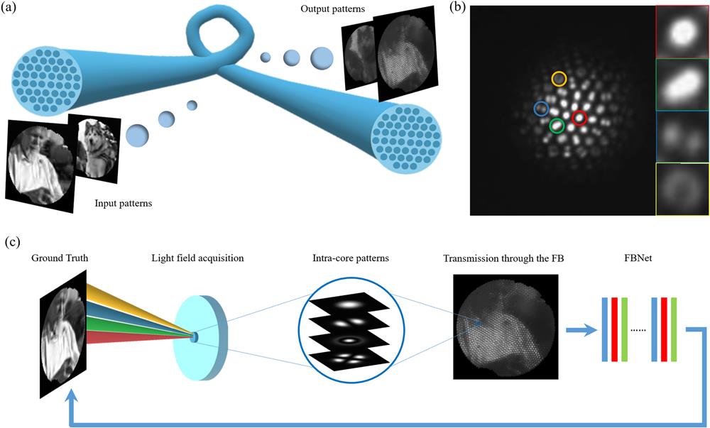
Fig. 1. Schematic of light field acquisition and feature enhancement reconstruction using the FB. (a) Changes in the images after transmission through the FB, where a completely clear image is split into multiple core patterns by the fiber core. (b) A snapshot of the proximal face of the FB when it is illuminated with a fiber probe at the distal. The colored circles highlight the different patterns excited by different incidence angles. A partial zoom-in view is shown on the right. (c) The imaging process uses the FB to acquire the light field including light field acquisition, transmission, and reconstruction via FBNet.

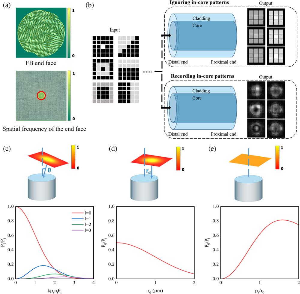
Fig. 2. Principle of light field acquisition using the FBs. (a) High-frequency light field information recorded in the core pattern. Up: spatial domain sampling of the FB. The yellow part corresponds to the fiber cores. Down: frequency domain sampling of the FB (given by the Fourier transform of the figure above). Low-frequency features are located in the center part of the image. Red circles correspond to the frequency of the core pitch size. (b) Sampling effect of different features smaller than the core size on the proximal end. Above: ignoring core features. Below: considering the in-core pattern. (c) On-axis Gaussian beam: the different color curves show the trend of the ratio of different excitation modes to the total incident power with an increasing angle of incidence. (d) Tilted Gaussian beam: the red curve shows the fundamental mode excitation efficiency as a function of a shift of a distance. (e) On-axis uniform beam: the red curve indicates the fundamental mode excitation efficiency as a function of the spot size of the beam and the modal.

Fig. 3. Neural network models and experimental setup. (a) Training procedure of the FBNet. The generator G learns to generate pseudo-real images in an attempt to fool the discriminator. Discriminator D learns to achieve classification between fake (synthesized by the generator) and real images. (b) FB image acquisition experimental setup diagram. The real image on the screen is displayed on the distal of the FB by a scaled combination of the lens (L1, f1=12mm) and objective (OBJ1, 50×). The pattern at the proximal of the FB is projected on the CMOS by a lens (L2, f2=30mm) and an objective (OBJ2, 40×).

Fig. 4. Results of training and testing of SM and FM using R-FBNet. The first row displays the original images recorded by the image sensor containing the mode patterns, their regions of interest, and the spatial frequency spectra. The results of reconstruction by the traditional interpolation method are shown in the second row. The third and fourth rows present the reconstruction results by R-FBNet for different datasets. Some boundary features are marked with orange circles. The ground truths (GTs) are listed in the last row as a comparison. The similarity coefficients of their spectrograms with the corresponding GTs are recorded in white.

Fig. 5. Results of training and testing of the SM and FM for textural features through U-FBNet. The first, second, and last rows illustrate the raw acquisition maps, the reconstruction maps by traditional methods, and the real images. The third and fourth rows show the results of the reconstructions using the SM and FM as the dataset, respectively. The regions of interest are enlarged by the color window, corresponding to a real image size of about 40 µm at the distal.

Fig. 6. Results of training and testing of the SM and FM for image colorization based on R-FBNet. The first row illustrates the raw SM and FM datasets used for image coloring. The colored maps and their saturation maps are shown in the second and third rows. The last row lists the GTs and their saturation graphs as a comparison. The white numbers indicate the similarity between the saturation of the reconstructed maps and the saturation of GTs.

Table 1. Comparison of Testing Results for Boundary Features

Table 2. Comparison of Testing Results for Textural Features

Table 3. Testing Results for Image Colorization