
Zhou Yuan, Meng Xiangqun, Jiang Dengbiao, Tang Houjun. Centerline Extraction of Structured Light Stripe Under Complex Interference[J]. Chinese Journal of Lasers, 2020, 47(12): 1204004
- Chinese Journal of Lasers
- Vol. 47, Issue 12, 1204004 (2020)
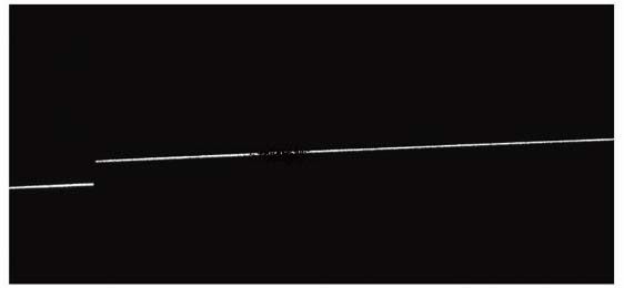
Fig. 1. Laser stripe that breaks due to surface contamination of the object being measured (simulation)
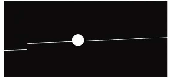
Fig. 2. Laser stripe disturbed by light spot (simulation)
Fig. 3. Laser stripe disturbed by sparks (simulation)
Fig. 4. Demonstration of density clustering algorithm. (a) Pixelated laser stripe image; (b) analysis of density clustering for local laser stripe image
Fig. 5. Pseudo-code of density clustering algorithm for binary image
Fig. 6. Demonstration of density clustering algorithm to repair broken stripe, ε=3, P=4
Fig. 7. Graph data structure based on core points
Fig. 8. Demonstration of broken stripe processing. (a) Enlarged view of simulated broken stripe interference; (b) experimental results on broken laser stripe
Fig. 9. Experimental results of light spot interference
Fig. 10. Experimental results of spark interference
Fig. 11. Enlarged view of the dotted framed area of Fig. 10
Fig. 12. Errors of different disturbed image extraction results relative to the reference centerline
Fig. 13. Extraction results of the proposed algorithm when applied to the actual stripe images. (a)--(d) Original images; (e)--(h) enlarged views
|
Table 1. Parameter setting of density clustering algorithm during experiment
|
Table 2. RMSE of the disturbed image extraction results relative to the reference centerlineunit:pixel
|
Table 3. Comparison of the average running time of different algorithmsunit:ms
|
Table 4. Comparison of the average running time of different algorithms used for practical imagesunit:ms

Set citation alerts for the article
Please enter your email address
© Copyright 2018-2021 | Chinese Laser Press. All Rights Reserved 沪ICP备15018463号-20