Net primary productivity (NPP) is the net carbon fixed by plants through photosynthesis (Wang et al., 2016; Huang et al., 2019). It is a key component of the terrestrial carbon cycle, which measures the direct production capacity of ecosystems (Schimel et al., 2001; Yuan et al., 2017). Besides, regional NPP is closely related to regional biodiversity, sustainability, and ecosystem security, and has been widely used to assess ecosystem vulnerability under climate change (Gao et al., 2017; Yuan et al., 2017). Therefore, the spatial and temporal characteristics of global and regional NPP have received wide attentions across the world (e.g., Woodward and Lomas, 2004; Doughty et al., 2015; Sun and Mu, 2018).

Several studies have been conducted examining NPP variations in China. For example, using the Atmosphere re-Vegetation Interaction Model, He et al. (2007) investigated the changes in terrestrial NPP in China during 1971-2000, and observed an increasing trend at a linear rate of 8.8 gC m^-2 dec^-1. Using the Integrated Biosphere Simulator (IBIS), Yuan et al. (2014) showed a reduction of NPP over most parts of eastern and central China, but found no significant trend for the country as a whole. There are also studies focusing on future changes in NPP in China. For example, Wang et al. (2016) evaluated NPP's variation over the 21st century based on earth system models in CMIP5, and showed an increasing trend of NPP over China under all four RCP scenarios, especially in western China. However, the increasing magnitude over western China is most variable across models, while it is pretty stable over eastern China. Huang et al. (2019) evaluated NPP variations based on the LPJ-DGVM model simulations, driven by various climate and CO₂ concentration scenarios in the 21st century. They found that the total NPP is projected to continuously increase under different scenarios, with CO₂ concentration playing the dominant role in driving the NPP increase in China. Using the LPJ-DGVM model, Sun and Mu (2018) confirmed that the NPP in China is expected to increase during 2011-2100 under RCP4.5.

Since the new scenarios of Shared Socioeconomic Pathways (SSPs) have been applied in CMIP6 (Eyring et al., 2016), the dynamics of future terrestrial ecosystems in China need to be re-evaluated. Moreover, the decline of regional NPP should receive more attentions than the increase of NPP, as it may lead to potential ecosystem crises. In this study, we adopt the SSP245 which is an only-one scenario of SSP2 implemented in the CMIP6 experiments. The SSP2 scenario represents a “middle of the road” scenario describing a future world that resembles the historical pattern the most (Riahi et al., 2017). The rest of the paper is organized as follows. Section 2 introduces the data and methods. Section 3 shows the main results, with discussions presented in Section 4. The main conclusions are summarized in Section 5.

The NPP and GPP were simulated by the second generation of Beijing Climate Center Climate System Model (BCC-CSM2) archived in the CMIP6 project. BCC-CSM is a global fully coupled climate-carbon cycle model (Wu et al., 2010; Wu et al., 2013), developed mainly for improving the simulation of China's climate (Xin et al., 2013; 2018; Wu et al., 2019). The first generation of BCC-CSM1.1 shows good performance in reproducing the observed atmospheric CO₂ concentration, and the interannual variability and long-term trend of global carbon cycle (Wu et al., 2013). BCC-CSM2 outperforms BCC-CSM1.1 in both the model resolution and physics (Wu et al., 2019). Taking the land surface model BCC-AVIM2.0 for example, several improvements are included on the basis of its predecessor BCC-AVIM1.0. BCC-AVIM2.0 employs a variable temperature threshold to determine soil water freezing-thawing instead of using a fixed temperature of 0℃ in BCC- AVIM1.0. Besides, BCC-AVIM2.0 adopts a better algorithm of snow surface albedo and snow cover fraction, a dynamic phenology for deciduous plant function types, and a four-stream approximation of solar radiation transfer through vegetation canopy (Li et al., 2019; Wu et al., 2019). All these contribute to the better performance in simulating vegetation phenology (Li et al., 2019). We use historical GPP/NPP simulations for the period 1980-2013, consistent with observations, and future projections for the period 2015-2100 under the SSP245 scenario. The climate data used in this study includes precipitation and near-surface air temperature for the historical period 1960-1999 and the future period 2015-2100. This historical period contains 40 years and is set the same as in Hempel et al. (2013). The historical simulations are compared with observations, based on which bias-correction of future projections is performed. All BCC-CSM2 simulations are available at the monthly scale at the T106 grid (approximately 110 km).

The observed monthly GPP at a spatial resolution of 0.5° is obtained from a gridded benchmark product upscaled from in situ FLUXNET measurements for the period 1980-2013 (Jung et al., 2009; 2011). The observation-constrained NPP fields are derived from GPP using the methodology described in the methods section. The monthly temperature and precipitation are obtained from the Climate Research Unit (CRU) (Harris et al., 2014) at a 0.5° spatial resolution from 1960-1999. All the 0.5° data are transformed into the BCC-CSM2 grid through bilinear interpolation before further analysis. There are many methods for spatial interpolation such as the nearest neighbor, inverse distance weighted, or Kriging etc. The bilinear interpolation method is chosen for its simplicity and representativeness.

2.2.1 Quantile mapping

Quantile mapping is a widely used approach in climate research for adjusting model results to match with observations (e.g., Themeßl et al., 2012; Maraun, 2013; Kim et al., 2016). It adjusts a model value at a given quantile from the cumulative distribution function (CDF) during the reference period to the observed value at the same quantile. The basic form is as:

where X_cor is the bias corrected value, X_mod is the model value, F is the cumulative distribution function, F^-1 is the inverse function of F. α and β are the shape and scale parameters, respectively. This study employs a non-parametric quantile mapping during the reference period, i.e., there is no specification of the probability distribution function for deriving the CDFs. Non-parametric quantile mapping shows better skill than parametric ones in reducing the systematic errors (Gudmundsson et al., 2012). For monthly GPP values lower than 0.1 g m^-2 mon^-1 and precipitation values lower than 0.1 mm mon^-1, a zero value is set to replace them. The quantile mapping parameters are then applied to adjust the future simulations of monthly GPP, temperature, and precipitation at each grid.

2.2.2 Derivation of NPP

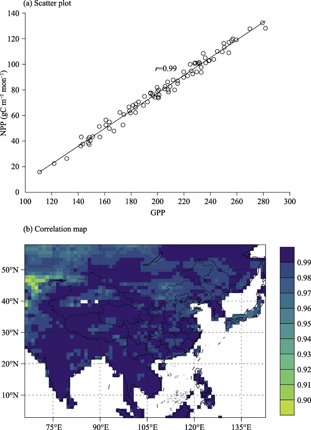
Since the FLUXNET product provides no observational NPP values, the future NPP cannot be corrected directly through quantile mapping. Nevertheless, given the close linear relationship between GPP and NPP (Figure 1) (e.g., Yu et al., 2013; Zhu et al., 2014; Wang et al., 2015), GPP can be used to derive NPP. The future GPP values from BCC-CSM2 are first bias-corrected through quantile mapping. Then, through linear regression of simulated NPP over GPP, a linear regression model is built at each grid for each month. With adjusted GPP, the adjusted NPP values are obtained through linear regressions. The linear regression expression is as:

where a and b are the regression coefficients of NPP over GPP, ε is the residual random error.

2.2.3 Piecewise linear regression model

The one-phase linear regression may not be sufficient to characterize the change features of NPP and climate (temperature and precipitation) during a long period. Thus, a two-phase piecewise regression method is adopted in this study to detect the potential change in the NPP time-series and identify the corresponding turning years. There are two forms of piecewise regression models (Wang et al., 2010): (1) non-continuous restriction at breakpoints; and (2) continuous at each breakpoint. Both have been widely used in the detection of temporal turning points (e.g., Menne and Williams, 2005; Piao et al., 2011; Zhang et al., 2018). Here the first kind of piecewise regression model is chosen to examine the temporal inhomogeneity, which is expressed as:

where y is dependent variable, t is the time, α₁, α₂, β₁ and β₂ are the regression coefficients, ε is the residual random error, n is the length of the time series, and c is the potential turning point. The least-squares linear regression is used to derive the estimators of c and other coefficients. The value of c that minimizes the following error function Q(c) is denoted as the turning year.

Compared with observations (Figure 2c), the modelled GPP (Figure 2a) has well reproduced the spatial pattern of “high southeast-low northwest” over China. Specifically, the integrated GPP value over China is 6.91 PgC a^-1 from BCC-CSM2 and 7.13 PgC a^-1 from FLUXNET during 1980-2013, indicating a well match between the two. Using non-parametric quantile mapping, the modelled GPP is adjusted to match the observations at grid scale. The adjusted GPP reproduces not only the long-term mean values of observations during the reference period (Figure 2b cf. Figure 2c), but also shows similar CDFs with the observation (Maraun, 2013). Compared with modelled GPP (Figure 2a), the locations with the highest GPP values are shifted southwestward from Zhejiang-Fujian provinces to Fujian-Guangxi provinces. The area with anomalously low GPP in central Hubei province is recovered with normal values. There are also other adjustments, such as the strengthening of GPP in Northeast China and west Xinjiang, and non-values over the major desert areas in Xinjiang and Inner Mongolia. These adjustments have made the simulated GPP more reasonable.

After the adjustment of future GPP, the linear regression parameters obtained from the modelled GPP and NPP at each grid (Figure 1) are applied to estimate the future NPP. The corrected annual NPP and its changing trend from 2015-2050 are shown in Figures 3b and 3d, respectively. NPP generally decreases from the southeast to the northwest over China, with some high values (over 1000 gC m^-2 a^-1) over Hubei-Hunan-Zhejiang and Yunnan provinces. In the original map without correction (Figure 3a), high values concentrate in the southeast of Zhejiang and Fujian and the southwest of Sichuan and Yunnan provinces.

The NPP shows a general increasing trend in the near-term in both the corrected and non-corrected simulations. However, the increasing magnitude of the non-corrected NPP is much larger than that of the corrected one (Figure 3c cf. 3d). It increases the most around the Sichuan Basin after correction. The increased NPP implies low risk to the terrestrial ecosystem in the near future. Similarly, the NPP shows a general increasing trend over China during 2015-2100 (Figure not shown). Compared with the historical situation, the projected NPP change seems to alleviate the worries on the potential ecosystem productivity crisis in the near future. However, ecosystem crisis may occur in the latter part of the century, which is hard to identify by the single-phase linear trend detection method. In light of this, the piecewise linear regression method is applied to detect the NPP changing trend in the latter part of the century.

The changing trend of NPP in the latter part of the 21st century (defined here as 2015-2100) is shown in Figure 4a. It exhibits more negative trend points over China, which are clustered spatially into three major regions, i.e., the northeast from east Inner Mongolia to Heilongjiang provinces, the central region from Gansu-Shaanxi to Hubei provinces, and the south from Zhejiang to Guangxi provinces. The south and the strip along the national boundary of Heilongjiang decrease the most, with the corresponding turning year shown in Figure 4b. In the northeast, NPP decreases primarily at two different years. Along the boundary strip, NPP decreases at around the year 2089. Inside China, NPP decreases around 2060. In the central region, the turning years vary widely without a uniform year. In the south, NPP generally decreases at around 2085. The grids with similar turning years and proximity in space are combined into two regions for regional analysis (in red boxes in Figure 4b), which are specified as the northeast region (NER) and the south region (SR), respectively. The time series of NPPs are shown in Figure 5. Through piecewise regression, the turning year for the NPP in NER falls in 2059, and 2085 in SR. NPP in NER increases at a rate of 1.6 gC m^-2 a^-1 dec^-1 insignificantly before 2059, but decreases significantly at the 0.05 level at a rate of -3.0 gC m^-2 a^-1 dec^-1 afterwards, equivalent to -0.9% dec^-1 of the long-term mean during 2059-2100. The NPP in SR increases at 3.1 gC m^-2 a^-1 dec^-1 before 2085, but decreases rapidly at -19.7 gC m^-2 a^-1 dec^-1 afterwards, both significant at the 0.01 level. The decreasing rate accounts for -2.4% dec^-1 of the mean from 2085-2100.

The correlation coefficients between NPP and the detrended temperature and precipitation from 2015-2100 are shown in Figures 6a and 6b. The BCC-CMS2 temperature and precipitation data have been bias-corrected against observations through quantile mapping. Temperature influences NPP differently over China. In the south and north of East China, temperature exerts a negative impact on NPP. As temperature increases unanimously over China in the 21st century under SSP245, a persistent negative effect on NPP over East China is expected. In the Tibetan Plateau and northern areas of Inner Mongolia and Heilongjiang provinces, temperature influences NPP positively, which is similar to the results based on IBIS (Yuan et al., 2014). Maybe it is because those areas are too cold for vegetation growth. Moderate temperature reduces there and remains as a primary constraint, and thus the persistent temperature increase in the future would benefit those regions. Precipitation influences NPP positively and significantly over most of China, except for some areas around Tibet.

To determine which climate factor is dominant in influencing NPP in different areas, the grids are divided into three categories according to the correlation parameters. The climate factor with larger correlation parameter r dominates the grid NPP. If both correlation parameters are significant at 0.05 level, the grid is marked with gray (Figure 6c). As a result, precipitation dominates the NPP variation over most of China in the 21st century, except for the Tibetan Plateau and Northeast China. In the central part around Shanxi and the southern part from Yunnan to Fujian, the ecosystems are influenced strongly by both precipitation and temperature.

To further reveal the abrupt negative change of regional NPP in NER and SR, the NPP series are compared with the corresponding climate series (Figure 7). These regional variables are standardized and linearly regressed before and after the turning year. In NER, NPP shifts from a weak increasing trend to a significant decreasing trend in 2059. However, the relevant climate factors do not show matching changes. Temperature after 2059 increases as before. Precipitation barely shows any trend either before or after 2059. Although a change point is detected for NPP in NER, it is hard to be attributed to the effects of climate variations. That said, the regional NPP is significantly related with both precipitation and temperature. The linear correlation parameters between NPP and the detrended temperature and precipitation for the 21st century are 0.18 (P<0.1) and 0.23 (P<0.05), respectively (Table 1).

In SR, a large portion of the areas is affected strongly by both precipitation and temperature (Figure 6c). Thus, the NPP change at the turning year of 2085 is probably due to the effects of the two climate factors. In SR, NPP turns from a significant increasing trend to a significant rapid decline at 2085, similar to that of the precipitation change. Temperature, however, drops at first, but rises again afterward. It is worth noticing that NPP is negatively related to temperature over SR (Figure 6a), with the correlation coefficient of -0.19 (P<0.10). Thus, the increase of temperature after 2085 serves as a secondary factor for the reduction of vegetation productivity in SR, while precipitation is the primary climate factor driving the negative NPP trend transition.

As GPP, temperature, and precipitation variables are bias-corrected separately through quantile mapping, the physical relations between NPP and climate in the model may be distorted (Hempel et al., 2013). The non-significant relations between NPP and climate in NER before and after 2059 may be due to the effects of separate bias-correction of the variables. To further explore this, the piecewise linear regression method is applied for the raw model data in NER, with the results shown in Figure 8. The original NPP still turns into negative in the year 2059. Temperature and precipitation show similar trend patterns before and after 2059 with those based on the adjusted data, confirming the minor influence of climate in regulating the NPP change. In addition, the relationship between climate and NPP has changed. The relationship between NPP and temperature becomes significant at 0.10 level after correction, while the relationship between NPP and precipitation weakens a bit (Table 1). This is consistent with the fact that in the humid and cold northeastern China, temperature is the major controlling factor for vegetation productivity. The bias correction seems to be more practical for the special case.

Using the BCC-CSM projections under the SSP245 scenario, the NPP change over China during the 21st century is analyzed in this study. We have reached the following conclusions.

(1) There are no risks in the terrestrial productivity in China in the near-term 2015-2050. NPP generally increases significantly over China, with the largest magnitude of increase in the Sichuan Basin.

(2) The ecosystem productivity risks may emerge in the latter part of the 21st century, as NPP is projected to decrease over three major regions, i.e., the northeast from eastern Inner Mongolia to Heilongjiang, the central region from southern Gansu to Chongqing-Hubei, and the south from Fujian to Guangxi. The turning year of NPP change in the central region varies strongly, while in the NER and SR regions, consistent turning years are detected. In NER, NPP decreases significantly after 2059 at a rate of -3.0 gC m^-2 a^-1 dec^-1, which accounts for -0.9% dec^-1 of the mean. In SR, NPP decreases rapidly after 2085 at -19.7 gC m^-2 a^-1 dec^-1, which accounts for -2.4% dec^-1 of the mean.

(3) NPP is strongly influenced by precipitation and temperature. The influence varies across China. The rapid NPP decline in SR is primarily attributed to the decline in precipitation, with temperature playing a secondary role. In NER, however, the NPP change seems to have no evident relations with climate variations.

It should be noted that the results are model-dependent, and thus, uncertainties arising from model structure and parameters are inevitable in addition to the complexity of terrestrial ecosystems. For example, NPP is closely related to precipitation. However, precipitation is a much more uncertain variable to project than temperature in climate models (Wang et al., 2016). As a result, the simulated NPP change would be largely affected by the uncertainties from precipitation. Further work should be done to examine the robustness of the projected NPP changes using multiple models constrained by observations.