Hyperspectral Remote Sensing Image Classification Algorithm Based on Nonlocal Mode Feature Fusion

Hongchao Liu; Anguo Dong

doi:10.3788/LOP57.061017

Journals >Laser & Optoelectronics Progress >Volume 57 >Issue 6 >Page 061017 > Article

Laser & Optoelectronics Progress
Vol. 57, Issue 6, 061017 (2020)

Hyperspectral Remote Sensing Image Classification Algorithm Based on Nonlocal Mode Feature Fusion

Hongchao Liu and Anguo Dong^*

Author Affiliations

School of Science, Chang'an University, Xi'an, Shaanxi 710064, China

show less

DOI: 10.3788/LOP57.061017 Cite this Article Set citation alerts

Hongchao Liu, Anguo Dong. Hyperspectral Remote Sensing Image Classification Algorithm Based on Nonlocal Mode Feature Fusion[J]. Laser & Optoelectronics Progress, 2020, 57(6): 061017 Copy Citation Text

show less

Fig. 1. Stack sparse auto-encoder model^[11]

Download full size

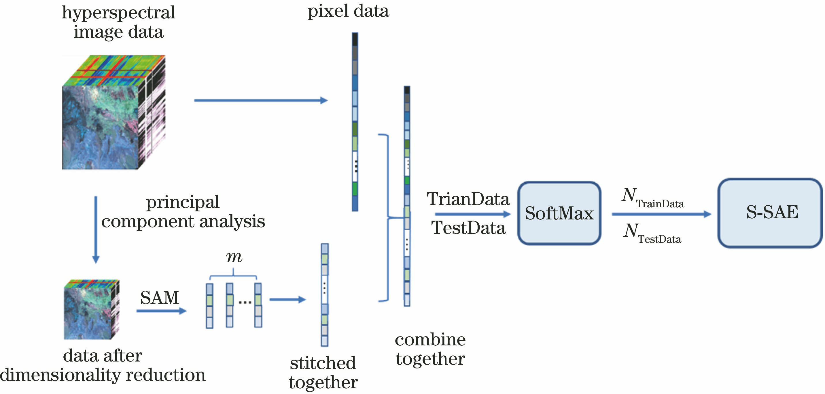
Fig. 2. Hyperspectral two-level classification model for nonlocal mode feature fusion

Download full size

Fig. 3. Classification results. (a) Classification results combined with local neighborhood information; (b) classification results combined with nonlocal mode feature fusion

Download full size

Fig. 4. Contrast figures before and after algorithm correction. (a) Before correction; (b) after correction

Download full size

Fig. 5. Classification results of Pavia University dataset obtained by different algorithms. (a) Original image; (b) true classification picture; (c) SVM; (d) CK-SVM; (e) SOMP; (f) MASR; (g) S-SAE; (h) our method

Download full size

Fig. 6. Classification results of Indian Pines dataset obtained by different algorithms. (a) Original image; (b) true classification picture; (c) SVM; (d) CK-SVM; (e) SOMP; (f)MASR; (g) S-SAE; (h) our method

Download full size

Fig. 7. Effect of number of training samples of different data on OA in different algorithms. (a) Pavia University; (b) Indian Pines

Download full size

Dataset	T
Dataset	0.96	0.97	0.98	0.99	0.999	0.9999
Indian Pines	86.95	87.54	88.46	90.14	95.37	97.86
Pavia University	93.95	94.52	95.16	96.14	98.55	99.12

Table 1. Relationship between imported label correctness rate and thresholdunit: %

Class	Number of samples		Classification accuracy /%
Class	Train	Test	SVM	CK-SVM	SOMP	MASR	S-SAE	Our method
Asphalt	200	6431	80.50	97.90	82.11	77.26	84.48	97.41
Meadows	200	18449	84.48	98.95	95.50	96.62	93.61	99.62
Gravel	200	1899	78.91	93.77	98.11	99.18	83.89	99.25
Trees	200	2864	96.24	98.96	96.24	96.91	98.43	98.64
Painted metal sheets	200	1145	99.74	100	99.06	100	100	100
Bare soil	200	4829	83.96	97.06	98.55	98.74	86.25	100
Bitumen	200	1130	91.39	99.56	98.34	99.99	87.79	100
Self-blocking bricks	200	3482	81.27	96.45	94.90	96.18	91.50	98.69
Shadows	200	747	98.44	99.87	88.44	83.59	99.74	99.95
OA/%			84.98	98.16	93.93	93.86	91.15	98. 61
Kappa			0.80	0.98	0.92	0.92	0.88	0.98

Table 2. Experimental data and classification accuracies of the Pavia University dataset

Class	Number of samples		Classification accuracy /%
Class	Train	Test	SVM	CK-SVM	SOMP	MASR	S-SAE	Our method
Alfalfa	5	41	60.47	74.42	83.72	88.83	68.83	93.56
Corn-notill	143	1285	68.53	84.75	90.58	98.24	82.18	97.13
Corn-mintill	83	747	59.01	85.03	90.10	97.82	79.03	96.49
Corn	23	214	38.22	86.67	92.89	95.07	81.91	97.57
Grass-pasture	50	433	92.16	100	91.27	97.48	95.99	96.23
Grass-trees	75	655	86.56	96.97	93.22	99.59	94.63	98.91
Grass-pasture-mowed	3	25	53.85	76.92	84.62	99.29	74.21	98.82
Hay-windrowed	49	429	94.26	99.78	99.78	99.96	98.19	98.99
Oats	2	18	22.22	94.44	44.44	69.00	92.86	94.34
Soybeans-notill	97	875	67.06	77.46	85.82	97.81	83.14	95.06
Soybeans-mintill	247	2208	73.17	93.41	94.86	98.63	92.47	98.03
Soybeans-clean	61	532	50.18	95.55	78.86	98.29	76.63	97.14
Wheat	21	184	94.85	99.48	90.21	98.74	99.25	99.40
Woods	129	1136	88.19	97.59	99.33	100	95.10	100
Bldg-grass-trees-drives	38	348	57.22	92.37	75.20	96.79	90.58	97.19
Stone-steel-towers	10	83	77.53	98.88	86.36	95.08	83.54	98.96
OA/%			73.01	91.36	91.46	97.41	88.67	97.35
Kappa			0.69	0.90	0.90	0.97	0.87	0.97

Table 3. Experimental data and classification accuracies of the Indian Pines dataset

Hongchao Liu, Anguo Dong. Hyperspectral Remote Sensing Image Classification Algorithm Based on Nonlocal Mode Feature Fusion[J]. Laser & Optoelectronics Progress, 2020, 57(6): 061017

Download Citation

Set citation alerts for the article

Tools

Set citation alerts for the article

Save the article for my favorites

Paper Information