Laterally swept light-sheet microscopy enhanced by pixel reassignment for photon-efficient volumetric imaging

Liang Qiao; Hongjin Li; Suyi Zhong; Xinzhu Xu; Fei Su; Xi Peng; Dayong Jin; Karl Zhanghao

doi:10.1117/1.APN.2.1.016001

Journals >Advanced Photonics Nexus >Volume 2 >Issue 1 >Page 016001 > Article

Advanced Photonics Nexus
Vol. 2, Issue 1, 016001 (2023)

Laterally swept light-sheet microscopy enhanced by pixel reassignment for photon-efficient volumetric imaging

Liang Qiao^1、†, Hongjin Li^1、2, Suyi Zhong³, Xinzhu Xu³, Fei Su^1、4, Xi Peng^1、3, Dayong Jin^1、4、*, and Karl Zhanghao^1、*

Author Affiliations

¹Southern University of Science and Technology, College of Engineering, UTS-SUSTech Joint Research Centre for Biomedical Materials and Devices, Department of Biomedical Engineering, Shenzhen, China

²City University of Hong Kong, Department of Biomedical Engineering, Hong Kong, China

³Peking University, College of Future Technology, Department of Biomedical Engineering, Beijing, China

⁴University of Technology Sydney, Institute for Biomedical Materials and Devices (IBMD), Faculty of Science, Sydney, Australia

show less

DOI: 10.1117/1.APN.2.1.016001 Cite this Article Set citation alerts

Liang Qiao, Hongjin Li, Suyi Zhong, Xinzhu Xu, Fei Su, Xi Peng, Dayong Jin, Karl Zhanghao. Laterally swept light-sheet microscopy enhanced by pixel reassignment for photon-efficient volumetric imaging[J]. Advanced Photonics Nexus, 2023, 2(1): 016001 Copy Citation Text

EndNote(RIS)

BibTex

Plain Text

show less

Schematic comparison between the ASLM and LSLM. (a) In the ASLM, a focused Gaussian beam is first laterally scanned that generates a light sheet perpendicular to the direction of beam propagation. Afterward, the focus of the Gaussian beam is axially swept in synchronization with the rolling shutter of the camera. In the LSLM, a Gaussian beam is first axially scanned that forms a “light needle” along the direction of beam propagation. Then, the beam is laterally swept in synchronization with the camera. Here, the axial direction is along the propagation of the beam and the lateral direction is perpendicular to the propagation of the beam. With the rolling shutter, only the region excited by the in-focus, thin light sheet is imaged by the camera. (b) Comparison of light sheets generated by lateral scanning of the ASLM and axial scanning of the LSLM. The images on the Y–Z plane show the cross section of the light sheet, and the yellow dashed lines indicate the rolling shutter. With the same rolling shutter, the ASLM shows better axial optical sectioning, but the LSLM contains more excitation power in the shutter region, which is more photon-efficient.

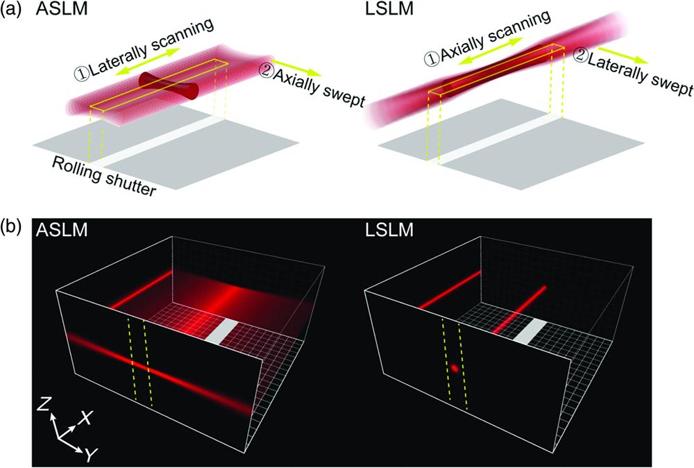
Fig. 1. Schematic comparison between the ASLM and LSLM. (a) In the ASLM, a focused Gaussian beam is first laterally scanned that generates a light sheet perpendicular to the direction of beam propagation. Afterward, the focus of the Gaussian beam is axially swept in synchronization with the rolling shutter of the camera. In the LSLM, a Gaussian beam is first axially scanned that forms a “light needle” along the direction of beam propagation. Then, the beam is laterally swept in synchronization with the camera. Here, the axial direction is along the propagation of the beam and the lateral direction is perpendicular to the propagation of the beam. With the rolling shutter, only the region excited by the in-focus, thin light sheet is imaged by the camera. (b) Comparison of light sheets generated by lateral scanning of the ASLM and axial scanning of the LSLM. The images on the

Y – Z

plane show the cross section of the light sheet, and the yellow dashed lines indicate the rolling shutter. With the same rolling shutter, the ASLM shows better axial optical sectioning, but the LSLM contains more excitation power in the shutter region, which is more photon-efficient.

Download full size | View in the Article

Comparison between the ASLM and LSLM with simulation studies. Cross-sectional view of the light sheet with a cropped Y-FoV of 100 μm in the Y–Z plane after the first scanning for (a) the ASLM and (b) the LSLM. The highlighted region shows an example of the rolling shutter with a width of ∼86.0 μm for the ASLM and ∼3.6 μm for the LSLM, for which the energy ratios are both ∼50% and the axial FWHM are both ∼1.2 μm for the two models. Scale bar: 10 μm. (c) Cross-sectional view of the SFLM in the Y–Z plane generated by lateral and axial scanning without confocal detection. (d) Intensity profiles along the Z axis for d1, d2, and d3. The FWHM is 0.81 μm for the ASLM, 0.88 μm for the LSLM, and 2.41 μm for the SFLM. (e) Intensity profiles along the Y axis for e1 and e2. (f) The energy ratio changes with rolling shutter widths for both the ASLM and LSLM. (g) The axial FWHM increases with a larger rolling shutter width for both the ASLM and LSLM. (h) Relationship between the axial FWHM and energy ratio.

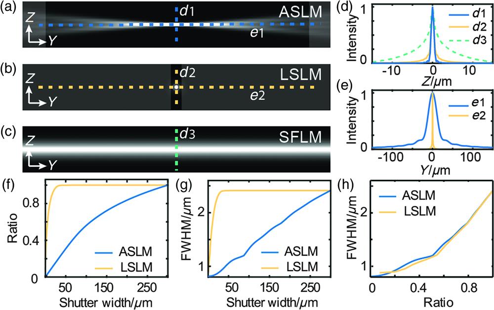
Fig. 2. Comparison between the ASLM and LSLM with simulation studies. Cross-sectional view of the light sheet with a cropped

Y

-FoV of

100 μ m

in the

Y – Z

plane after the first scanning for (a) the ASLM and (b) the LSLM. The highlighted region shows an example of the rolling shutter with a width of

\sim 86.0 μ m

for the ASLM and

\sim 3.6 μ m

for the LSLM, for which the energy ratios are both

\sim 50 %

and the axial FWHM are both

\sim 1.2 μ m

for the two models. Scale bar:

10 μ m

. (c) Cross-sectional view of the SFLM in the

Y – Z

plane generated by lateral and axial scanning without confocal detection. (d) Intensity profiles along the

Z

axis for

d_{1}

d_{2}

, and

d_{3}

. The FWHM is

0.81 μ m

for the ASLM,

0.88 μ m

for the LSLM, and

2.41 μ m

for the SFLM. (e) Intensity profiles along the

Y

axis for

e_{1}

and

e_{2}

. (f) The energy ratio changes with rolling shutter widths for both the ASLM and LSLM. (g) The axial FWHM increases with a larger rolling shutter width for both the ASLM and LSLM. (h) Relationship between the axial FWHM and energy ratio.

Download full size | View in the Article

Fig. 3. Simulated imaging results of fluorescent beads. (a) and (b) Simulated imaging results of fluorescence beads in the

X – Y

and

X – Z

planes, and the three insets show the imaging results of the white dashed areas in the ASLM, iLSLM, and SFLM. (c) The upper and lower parts show the profiles of the ASLM, iLSLM, and SFLM when the photon efficiencies reach 58% and 80%, respectively. (d) and (e) Simulations to compare the photon efficiency and the axial FWHM of the ASLM and iLSLM with increasing rolling shutter. (f) Relationship between photon efficiency and the axial FWHM of the ASLM and iLSLM. Scale bar:

10 μ m

Download full size | View in the Article

Fig. 4. The microscopy setup and focus scanning with the SLM. (a) Schematic diagram of the light sheet microscope. Laser: 473 nm, bandwidth 0.2 nm, MBL-III-473, CNI;

L_{1} - L_{3}

: achromatic plano-convex lens,

L_{1} = 50 mm

L_{2} = 250 mm

L_{3} = 250 mm

; HWP1 and HWP2: half-wavelength plate, WPA2420-450-650, Union Optic; PBS, polarization beam splitter; CCM1-PBS251/M, Thorlabs; SLM, spatial light modulator, QXGA-R11, ForthDD; EO: excitation objective Lens, 20X/N.A. W, Olympus; DO: detection objective Lens, 10X/N.A. W, Olympus; Filter: ET525/50 M, Chroma; TL: tube lens, 200 mm, C60-TUBE B, ASI; Camera: ORCA-Flash 4.0, Hamamatsu. (b) and (c) When a binary phase pattern is loaded onto the SLM, the focus of the beam can be scanned in three dimensions. (d) Corresponding images when different phase patterns are loaded onto the SLM.

Download full size | View in the Article

Fig. 5. Experimental imaging results of fluorescent beads and U2OS cells. (a) and (b) Experimental imaging results of fluorescence beads in the

X – Y

and

X – Z

planes, and the three insets show the imaging results of the white dashed areas in the ASLM, iLSLM, and SFLM. (c) The upper and lower parts show the profiles of the ASLM, iLSLM, and SFLM when the photon efficiencies reach 58% and 80%, respectively. (d) and (e) The photon efficiency and axial FWHM of the ASLM and iLSLM corresponding to the increasing rolling shutter. (f) Relationship between the photon efficiency and the axial FWHM of the ASLM and the iLSLM. (g)–(i) The ASLM and iLSLM imaging results of U2OS cells corresponding to the photon efficiencies of 53% and 80%. Scale bar: