Remote Sensing Image Segmentation Using Super-Pixel and Dot Product Representation of Graphs

Daming Zhang; Xueyong Zhang; Huayong Liu; Lu Li

doi:10.3788/LOP202259.1210015

Journals >Laser & Optoelectronics Progress >Volume 59 >Issue 12 >Page 1210015 > Article

Laser & Optoelectronics Progress
Vol. 59, Issue 12, 1210015 (2022)

Remote Sensing Image Segmentation Using Super-Pixel and Dot Product Representation of Graphs

Daming Zhang^1、2、*, Xueyong Zhang^1、2, Huayong Liu¹, and Lu Li¹

Author Affiliations

¹School of Mathematics & Physics, Anhui Jianzhu University, Hefei 230022, Anhui , China

²Key Laboratory of Architectural Acoustic Environment of Anhui Higher Education Institutes, Hefei 230601, Anhui , China

show less

DOI: 10.3788/LOP202259.1210015 Cite this Article Set citation alerts

Daming Zhang, Xueyong Zhang, Huayong Liu, Lu Li. Remote Sensing Image Segmentation Using Super-Pixel and Dot Product Representation of Graphs[J]. Laser & Optoelectronics Progress, 2022, 59(12): 1210015 Copy Citation Text

show less

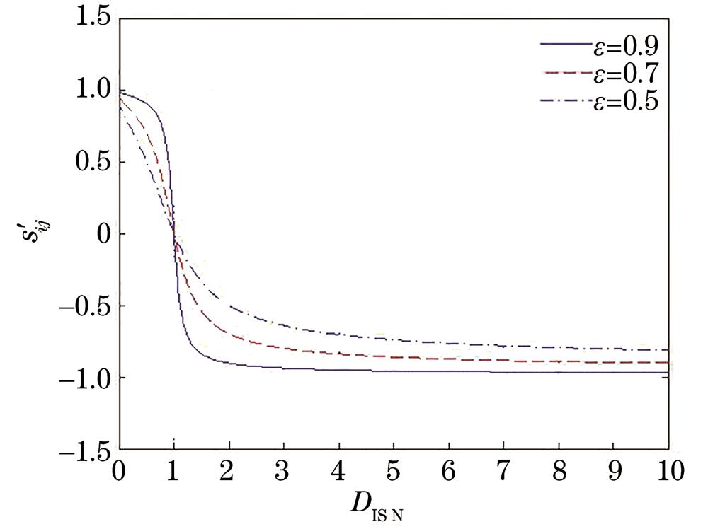
Fig. 1. Graph of function

\frac{2}{π} a r c t a n (l n {D_{I S}}_{N} / l n ε)

Download full size

Experimental results of Swiss Roll data. (a) Original data; (b) dimensionality reduction data before correction; (c) dimensionality reduction data after correction

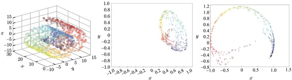
Fig. 2. Experimental results of Swiss Roll data. (a) Original data; (b) dimensionality reduction data before correction; (c) dimensionality reduction data after correction

Download full size

Fig. 3. Experimental results of UMIST Face Database. (a) Original data; (b) dimensionality reduction data before correction; (c) dimensionality reduction data after correction

Download full size

Fig. 4. Flow chart of the proposed multispectral remote sensing image segmentation algorithm

Download full size

Fig. 5. Experiment 1. (a) Original image; (b) Ground Truth

Download full size

Fig. 6. Segmentation results under parameter q in experiment 1. (a) q=5; (b) q=10; (c) q=20; (d) q=50; (e)‒(h) corresponding segmentation results

Download full size

Fig. 7. Segmentation results of experiment 2. (a) Original image; (b) Ground Truth; (c) segmentation result of SLIC; (d) segmentation result of proposed algorithm before correction; (e) segmentation result of proposed algorithm after correction

Download full size

Fig. 8. Segmentation results of experiment 3

Download full size

Fig. 9. Segmentation results of experiment 4

Download full size

Input：data set $Y = [y_{1}, y_{2}, \dots, y_{n}] \in R^{p \times n}$ ；similarity matrix $S \in R^{n \times n}$ ；positive integer $d$ Output：matrix $X = [x_{1}, x_{2}, \dots, x_{n}] \in R^{d \times n}$
1. Initialize matrix $D$ to be $n \times n$ zero matrix
2. $S = S + D$
3. Compute the dth largest eigen-values $λ_{i}$ of matrix $S$ and the corresponding eigen-vectors $μ_{i}$ ， $i = 1, \dots, d$
4. Let $X = [x_{1}, x_{2}, \dots, x_{n}]$ ，where
$x_{j} = {(\sqrt[]{λ_{1}} μ_{1 j}, \dots, \sqrt[]{λ_{n}} μ_{n j})}^{T}$ ， $j = 1, \dots, n$
5. Let $D = I \circ X^{T} X$ ，where $I$ is identity matrix， $\circ$ is multiplication that elements of matrix multiplied by elements of matrix
6. Turn to step 2. until convergence
7. Output matrix $X$

Table 1. Flowchart of dot product representation of graphs

Parameter	Before modification	After modification
Distance	$D_{I S}$	${D_{I S}}_{N} = D_{I S} / T_{t h r e s h o l d}$
Range of similarity	$s_{i j} \in [0,1]$	$s_{i j}^{'} \in [- 1,1]$
Range of angular	$θ_{i j} \in [0, π / 2]$	$θ_{i j}^{'} \in [0, π]$
Calculation formula	$s_{i j} = e x p (- {‖y_{i} - y_{j}‖}^{2} / 2 σ^{2})$	$s_{i j}^{'} = \frac{2}{π} a r c t a n (l n {D_{I S}}_{N} / l n ε)$

Table 2. Similarity before modification versus similarity after modification

Parameter	q= $5$	q= $10$	q= $20$	q= $50$
Precision	0.8729	0.8698	0.8236	0.7172
Recall	0.8763	0.8791	0.8367	0.7461

Table 3. Evaluation results of experiment 1

Parameter	Before correction	After correction
Precision	0.7729	0.8651
Recall	0.8132	0.9264

Table 4. Evaluation results of experiment 2

Parameter	FNEA（100）	FNEA（150）	MCG	Proposed algorithm（ $K = 7$ ）	Proposed algorithm（ $K = 4$ ）
Precision	0.7729	0.7548	0.8498	0.8592	0.8636
Recall	0.8761	0.8827	0.9563	0.9681	0.9507

Table 5. Evaluation results of experiment 3

Parameter	FNEA（50）	FNEA（100）	MCG	Proposed algorithm（ $K = 7$ ）	Proposed algorithm（ $K = 4$ ）
Precision	0.7149	0.7283	0.8559	0.8337	0.8472
Recall	0.8132	0.8362	0.9317	0.9119	0.9326

Table 6. Evaluation results of experiment 4

Download Citation

Set citation alerts for the article

Tools

Set citation alerts for the article

Save the article for my favorites

Paper Information