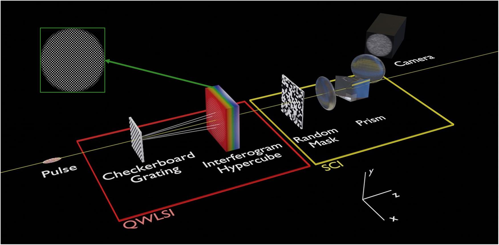
Fig. 1. Schematic of the experimental setup that was simulated. The pulse first travels through a quadriwave lateral shearing interferometer, yielding a hypercube of interferograms, a slice of which is shown in the green box. The hypercube is then passed through a CASSI setup. This consists of a random mask and a relay system encompassing a prism, before the coded shot is captured with the camera. This diagram is not to scale.

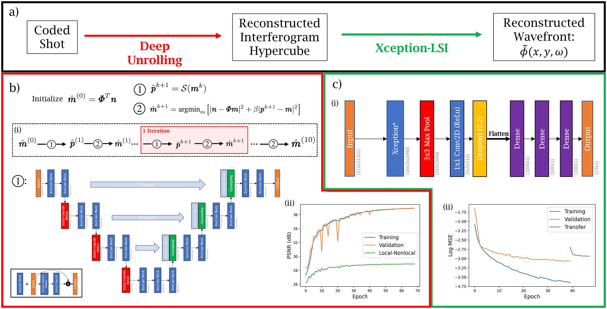
Fig. 2. A diagram showing the full reconstruction process of the wavefront from the coded shot. (a) A flow chart of the reconstruction process. (b) (i) The deep unrolling process, where sub-problems ① and ② are solved recursively for 10 iterations. Also shown is the neural network structure used to represent . (ii) The training curve for the deep unrolling algorithm. Plotted is the training and validation PSNR for the 3D ResUNet prior that was used, as well as the validation score for a local–nonlocal prior. Here is demonstrated the superior power of 3D convolutions in this setting. (i) The network design for the Xception-LSI network. The Xception* block represents that the last two layers were stripped from the conventional Xception network. (c) (ii) The training curve for Xception-LSI for training and validation sets, with the loss shown in log mean squared error. Also plotted is the validation loss when further training the model on the deep unrolling reconstruction of the data (transfer).

Fig. 3. Example results of the reconstruction process. (a) An example of the coded shot, along with a zoomed section. (b) Deep unrolling reconstruction of the interferogram hypercube in the same zoomed section at different wavelength slices. (c) The Xception-LSI reconstruction of the spatio-spectral wavefront displayed in terms of Zernike coefficients, where the x-axis of each plot is the Zernike function, the y-axis is the wavelength and the colour represents the value of the coefficient. (d) The spatial wavefront resulting from a Zernike basis expansion of the coefficients in (c) at the labelled spectral channels.