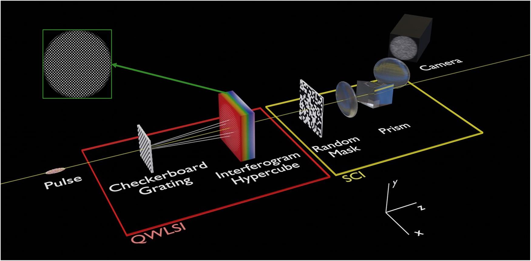
Presented is a novel way to combine snapshot compressive imaging and lateral shearing interferometry in order to capture the spatio-spectral phase of an ultrashort laser pulse in a single shot. A deep unrolling algorithm is utilized for snapshot compressive imaging reconstruction due to its parameter efficiency and superior speed relative to other methods, potentially allowing for online reconstruction. The algorithm’s regularization term is represented using a neural network with 3D convolutional layers to exploit the spatio-spectral correlations that exist in laser wavefronts. Compressed sensing is not typically applied to modulated signals, but we demonstrate its success here. Furthermore, we train a neural network to predict the wavefronts from a lateral shearing interferogram in terms of Zernike polynomials, which again increases the speed of our technique without sacrificing fidelity. This method is supported with simulation-based results. While applied to the example of lateral shearing interferometry, the methods presented here are generally applicable to a wide range of signals, including Shack–Hartmann-type sensors. The results may be of interest beyond the context of laser wavefront characterization, including within quantitative phase imaging.