
Zezheng Qin, Mingjian Sun, Yiming Ma, Zhigang Lei, Yuanyuan Gao. Intelligent Denoising Algorithm for Signals Based on Three-Dimensional Photoacoustic Tomography System[J]. Laser & Optoelectronics Progress, 2022, 59(8): 0811006
- Laser & Optoelectronics Progress
- Vol. 59, Issue 8, 0811006 (2022)
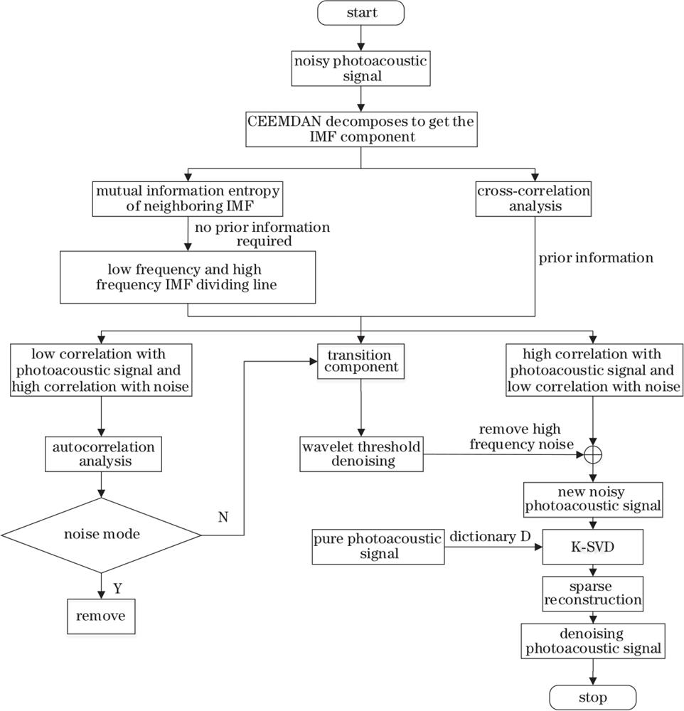
Fig. 1. Overall flow chart of proposed algorithm
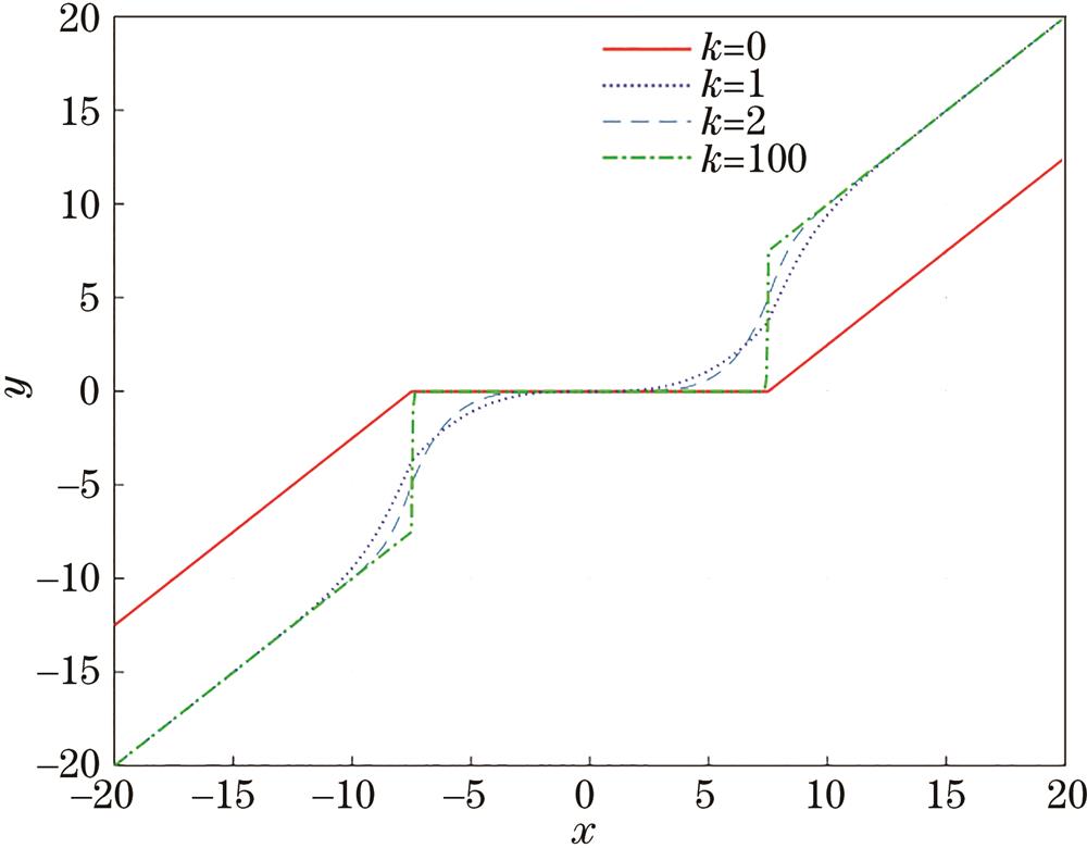
Fig. 2. New threshold processing function
Fig. 3. Comparison diagrams of different threshold functions. (a) Original signal; (b) noisy signal; (c) soft threshold denoising function; (d) proposed threshold denoising function; (e) hard threshold denoising function
Fig. 4. Comparison of noisy photoacoustic signal and pure photoacoustic signal. (a) Pure photoacoustic signal;(b) noisy photoacoustic signal
Fig. 5. Decomposition diagram of CEEMDAN
Fig. 6. Analysis of mutual information entropy of adjacent IMF components
Fig. 7. Correlation analysis
Fig. 8. IMF11 autocorrelation analysis
Fig. 9. Dictionary atoms constituting pure photoacoustic signals
Fig. 10. Denoising effect of proposed algorithm
Fig. 11. Comparison of denoising effects of different denoising algorithms
Fig. 12. Comparison of time-frequency domain analysis of photoacoustic signals for different denoising algorithms. (a) Denoising results of different denoising algorithms; (b) time-frequency distributions of photoacoustic signals based on different denoising algorithms
Fig. 13. Comparison of imaging effects after denoising: (a) Photoacoustic image generated by pure photoacoustic signal; (b) photoacoustic image generated by noisy photoacoustic signal; (c) photoacoustic image after denoising.
Fig. 14. Top view of full irradiated light path
Fig. 15. Schematic diagram of photoacoustic tomography system
Fig. 16. Photoacoustic tomography system
Fig. 17. Phantom to be scanned and scanning position. (a) Tumor mimicry ; (b) scanning rendering; (c) enlarged effect diagram of dotted frame
Fig. 18. Comparison of denoising effects. (a) Noisy photoacoustic signal reconstruction image; (b) photoacoustic signal reconstruction after denoising
Fig. 19. Photoacoustic imaging of each section and three-dimensional photoacoustic imaging effect. (a) Photoacoustic images of 42 sections; (b) three-dimensional photoacoustic imaging of tumor mimicry
|
Table 1. Comparison of photoacoustic image parameters before and after denoising
| |||||||||||||||||||||||||||||||||||||||||||||||||||||||||||
Table 2. Comparison of photoacoustic image parameters before and after denoising

Set citation alerts for the article
Please enter your email address
© Copyright 2018-2021 | Chinese Laser Press. All Rights Reserved 沪ICP备15018463号-20