
Yizhou Qian, Zhiyong Yang, Yu-Hsin Huang, Kuan-Heng Lin, Shin-Tson Wu. Directional high-efficiency nanowire LEDs with reduced angular color shift for AR and VR displays[J]. Opto-Electronic Science, 2022, 1(12): 220021
- Opto-Electronic Science
- Vol. 1, Issue 12, 220021 (2022)
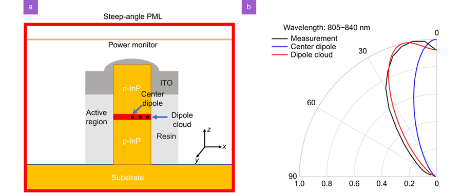
Fig. 1. (a ) 3D-FDTD InP nanowire LED simulation schematic. (b ) Simulated far-field radiation patterns of InP nanowire LED. The experimental data (black curve) included for comparison are from ref.31.
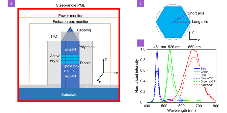
Fig. 2. (a ) Schematic of FDTD simulation model in x-z plane. (b ) Top view of blue hexagonal nanowire LED. (c ) Measured EL spectra of single nanowire LEDs with different diameters from ref.25.
Fig. 3. (a –c ) Normalized 2D angular distribution for (a) blue, (b) green, and (c) red LEDs. (d ) Normalized 1D angular distribution when azimuthal angle φ=0°.
Fig. 4. (a ) Simulated color triangle of the GaN/InGaN nanowire LED display and CIE coordinates of 18 reference colors at 0° viewing angle. (b ) Simulated color shift of 18 reference colors from 0° to 20° viewing angle. Inset: Simulated average color shift from 0° to 30° viewing angle.
Fig. 5. (a –c ) 2D colormap of angular FWHM as a function of n-GaN thickness and p-GaN capping height: (a) blue, (b) green, and (c) red nanowire LEDs. (d –f ) 2D colormap of effective LEE as a function of n-GaN thickness and p-GaN capping height: (d) blue, (e) green, and (f) red nanowire LEDs.
Fig. 6. (a –c ) Normalized 2D angular distribution for optimized (a) blue, (b) green, and (c) red LEDs. (d ) Comparison of normalized 1D angular distribution between unoptimized (solid lines) and optimized (dashed lines) nanowire LEDs.
Fig. 7. Comparison between calculated effective EQE of nanowire LED (horizontal dash lines) with measured EQE of (a ) blue InGaN µLEDs from ref.9,43, (b ) green InGaN µLEDs from ref.43-47 and (c ) red AlGaInP µLEDs from ref.48 as a function of mesa diameter. Vertical dash lines: EQE of µLEDs with 10-µm mesa size.
Fig. 8. (a ) Simulated angular color shift of 18 reference colors from 0° to 20° after optimization. (b ) Simulated average color shift from 0° to 30° viewing angle after optimization.


Set citation alerts for the article
Please enter your email address

© Copyright 2018-2021 | Chinese Laser Press. All Rights Reserved 沪ICP备15018463号-20