Author Affiliations
1School of Opto-electronic Engineering, Changchun University of Science and Technology, Changchun 130022, China2Science and Technology High-precision Optoelectronic Measurements Industry Technology Research and Development Center of Changchun City, Changchun 130022, China3Changchun Railway Vehicles Co., LTD., Changchun 130062, Chinashow less
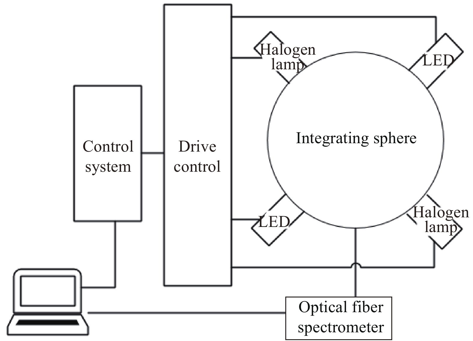
Fig. 1. System composition diagram
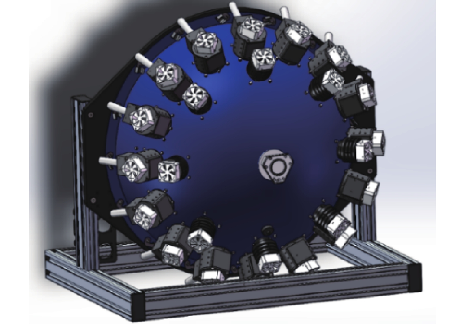
Fig. 2. Integrating sphere structure diagram
Fig. 3. Spectral radiance curve of bromine tungsten lamp
Fig. 4. Spectral curve of selected LED
Fig. 5. Illuminance formed by the surface light source on the surface at the distance r
Fig. 6. LED constant current drive circuit
Fig. 7. Convergence graph of simulated color temperature 5 500 K
Fig. 8. Simulation results of 5 500 K color temperature
Fig. 9. Experiment site of star simulator light source simulation
Fig. 10. Software control interface
Fig. 11. Spectral fitting curve of 5 500 K color temperature for 2nd magnitude sta
| Color temperature
magnitude
| 3 000 K/
(W/m2)
| 4 300 K/
(W/m2)
| 5 500 K/
(W/m2)
| 6 500 K/
(W/m2)
| 7 600 K/
(W/m2)
| 20 000 K/
(W/m2)
| | +2Mi | 4.29×10⁻⁹ | 2.81×10⁻⁹ | 2.47×10⁻⁹ | 2.36×10⁻⁹ | 2.32×10⁻⁹ | 2.37×10⁻⁹ | | +3Mi | 1.71×10⁻⁹ | 1.12×10⁻⁹ | 9.82×10⁻¹⁰ | 9.40×10⁻¹⁰ | 9.22×10⁻¹⁰ | 9.42×10⁻¹⁰ | | +4Mi | 6.79×10⁻¹⁰ | 4.46×10⁻¹⁰ | 3.91×10⁻¹⁰ | 3.74×10⁻¹⁰ | 3.67×10⁻¹⁰ | 3.75×10⁻¹⁰ | | +5Mi | 2.70×10⁻¹⁰ | 1.77×10⁻¹⁰ | 1.56×10⁻¹⁰ | 1.49×10⁻¹⁰ | 1.46×10⁻¹⁰ | 1.49×10⁻¹⁰ | | +6Mi | 1.08×10⁻¹⁰ | 7.06×10⁻¹¹ | 6.20×10⁻¹¹ | 5.93×10⁻¹¹ | 5.82×10⁻¹¹ | 5.95×10⁻¹¹ | | +7Mi | 4.28×10⁻¹¹ | 2.81×10⁻¹¹ | 2.47×10⁻¹¹ | 2.36×10⁻¹¹ | 2.32×10⁻¹¹ | 2.37×10⁻¹¹ | | +8.5Mi | 1.08×10⁻¹¹ | 7.06×10⁻¹² | 6.21×10⁻¹² | 5.92×10⁻¹² | 5.81×10⁻¹² | 5.94×10⁻¹² |
|
Table 1. Irradiance at the exit of the collimator
| Color temperature
magnitude
| 3 000 K
/W/(m2·sr)
| 4 300 K
/W/(m2·sr)
| 5 500 K
/W/(m2·sr)
| 6 500 K
/W/(m2·sr)
| 7 600 K
/W/(m2·sr)
| 20 000 K
/W/(m2·sr)
| | +2Mi | 307.31 | 201.29 | 176.93 | 169.05 | 166.19 | 169.77 | | +3Mi | 122.49 | 80.23 | 70.34 | 67.33 | 66.05 | 67.48 | | +4Mi | 48.64 | 31.95 | 28.01 | 26.79 | 26.29 | 26.86 | | +5Mi | 19.34 | 12.68 | 11.18 | 10.67 | 10.46 | 10.67 | | +6Mi | 7.71 | 5.06 | 4.44 | 4.25 | 4.17 | 4.26 | | +7Mi | 3.07 | 2.01 | 1.77 | 1.69 | 1.66 | 1.70 | | +8.5Mi | 0.774 | 0.506 | 0.445 | 0.424 | 0.416 | 0.426 |
|
Table 2. Radiance at the exit of the integrating sphere
| Number | Algorithm | Advantages | Disadvantages | | 1 | Genetic algorithm | Main steps of the genetic algorithm include selection, crossover and mutation. It can be seen that the algorithm
has a simple structure, does not rely on complex models,
and has no requirements on the continuity and
differentiability of the objective function
| It has the local search ability, but the global search ability is not strong, and it is easy to fall
into the local optimal
| | 2 | Ant colony algorithm | Results obtained by ant colony algorithm do not depend on
the choice of the initial route, and its parameters are few,
the setting is simple and easy to be combined
with other algorithms
| There is no clear theoretical basis for the parameter setting of ant colony algorithm, most of which is determined by experience and experiment | | 3 | Quantum particle swarm optimization | Global convergence is good, the global search ability is strong, the particle position is random, will not fall into the global optimal solution, the algorithm itself execution time is short | Difficulty in parameter selection | | 4 | Least square method | Calculation is simple and easy to be realized by
simple program of computer
| Least square method is a linear estimation with certain limitations and low optimization accuracy. In the process of regression, it is impossible for the correlation formula of regression to pass every regression data point | | 5 | Simulated annealing algorithm | Calculation process is simple, universal and has strong sculling ability. It is suitable for parallel processing and can be used to
solve complex nonlinear optimization problems
| Algorithm convergence speed is slow, the running time is long, the algorithm
performance is related to the initial value,
the parameter is sensitive
|
|
Table 3. Advantages and disadvantages of the five algorithms
| Magnitude
color temperature
| +2Mi | +3Mi | +4Mi | +5Mi | +6Mi | +7Mi | +8.5Mi | | 3 000 K | 2.40% | 2.25% | 2.53% | 2.08% | 2.17% | 2.82% | 3.87% | | 4 300 K | 2.67% | 2.95% | 3.23% | 3.56% | 3.40% | 3.98% | 4.58% | | 5 500 K | 3.51% | 3.96% | 4.54% | 4.82% | 5.40% | 5.93% | 6.14% | | 6 500 K | 3.75% | 4.11% | 4.96% | 4.87% | 5.92% | 6.23% | 6.74% | | 7 600 K | 3.65% | 4.56% | 5.03% | 5.45% | 6.33% | 6.87% | 7.10% | | 20 000 K | 5.10% | 5.90% | 6.70% | 8.10% | 8.80% | 9.60% | 9.80% |
|
Table 4. Spectral matching error
| Color temperature
magnitude
| 3 000 K/
W/(m2·sr)
| 4 300 K/
W/(m2·sr)
| 5 500 K/
W/(m2·sr)
| 6 500 K/
W/(m2·sr)
| 7 600 K/
W/(m2·sr)
| 20 000 K/
W/(m2·sr)
| | +2Mi | 307.26 | 200.05 | 179.31 | 167.12 | 163.54 | 167.49 | | +3Mi | 123.23 | 81.98 | 69.01 | 69.03 | 64.68 | 65.21 | | +4Mi | 48.02 | 30.56 | 27.01 | 26.06 | 26.92 | 27.77 | | +5Mi | 19.86 | 13.22 | 11.67 | 11.10 | 10.09 | 10.28 | | +6Mi | 7.46 | 5.21 | 4.26 | 4.00 | 3.99 | 4.54 | | +7Mi | 3.17 | 1.94 | 1.68 | 1.78 | 1.75 | 1.79 | | +8.5Mi | 1.27 | 0.844 | 0.666 | 0.711 | 0.698 | 0.714 |
|
Table 5. Measured radiance
| Color temperature
magnitude
| 3 000 K/
W·(m2·sr)
| 4 300 K/
W/(m2·sr)
| 5 500 K/
W/(m2·sr)
| 6 500 K/
W/(m2·sr)
| 7 600 K/
W/(m2·sr)
| 20 000 K/
W/(m2·sr)
| | +2Mi | 0.84% | −0.97% | 1.31% | −1.11% | −1.48% | −1.47% | | +3Mi | 1.00% | 2.22% | −1.97% | 2.42% | −2.15% | −3.39% | | +4Mi | −1.40% | −4.2% | −3.53% | −2.76% | 2.35% | 3.23% | | +5Mi | 2.37% | 4.09% | 4.20% | 3.74% | −3.90% | −3.93% | | +6Mi | −3.24% | 2.96% | −4.05% | 4.25% | 4.17% | 4.26% | | +7Mi | 3.26% | −3.48% | −5.08% | 5.33% | 5.42% | 5.29% | | +8.5Mi | 4.10% | 5.24% | −5.40% | 5.49% | 5.76% | 5.78% |
|
Table 6. Magnitude simulation accuracy
| Time | Radiation brightness /W/(m2·sr)
| | 9:00 | 10.73 | | 10:00 | 10.88 | | 11:00 | 11.01 | | 12:00 | 10.91 | | 13:00 | 10.75 | | 14:00 | 10.84 |
|
Table 7. Radiance after 6 hours of continuous work