
Zexing Du, Jinyong Yin, Jian Yang. Remote Sensing Aircraft Image Detection Based on Semi-Supervised Learning[J]. Laser & Optoelectronics Progress, 2020, 57(6): 061009
- Laser & Optoelectronics Progress
- Vol. 57, Issue 6, 061009 (2020)
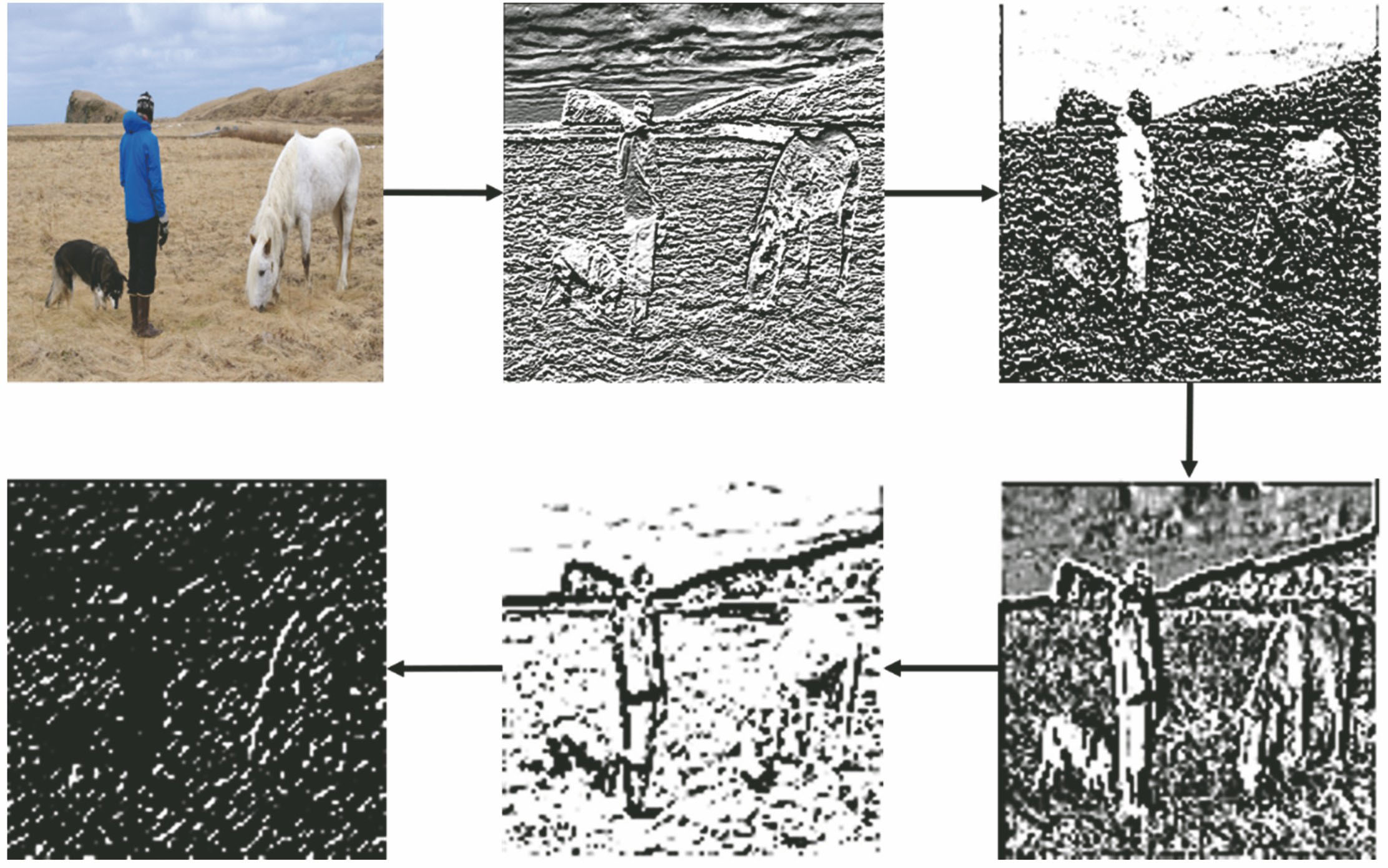
Fig. 1. Information extracted by the convolutional structure of each layer in CNN structure
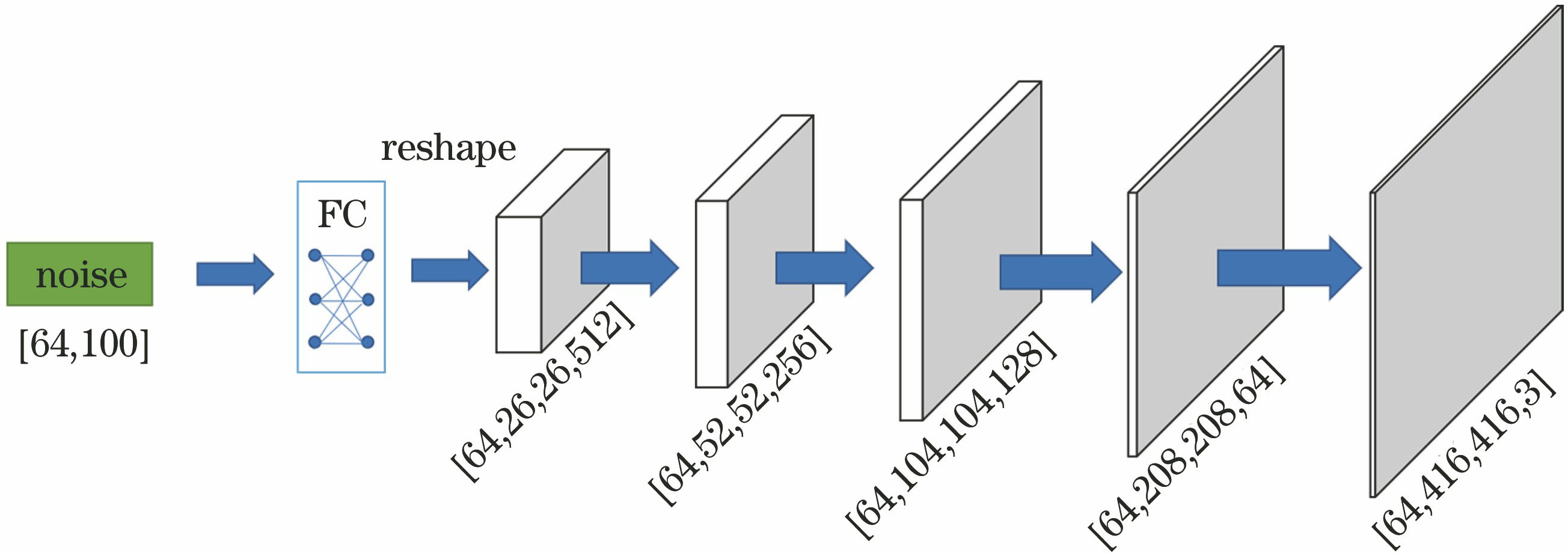
Fig. 2. Generator network model for coarse-grained network
Fig. 3. Discriminator network model for coarse-grained network
Fig. 4. Discriminator network model for fine-grained network
Fig. 5. Extracted objects to be detected by tailoring
Fig. 6. Model of object detection network
Fig. 7. Part of dataset
Fig. 8. Loss function values for different models in coarse-grained network. (a) Discriminator network; (b) generator network
Fig. 9. Loss function values for different models in fine-grained network. (a) Discriminator network; (b) generator network
Fig. 10. Airplane images produced by fine-grained network
Fig. 11. Change in loss function value during the training process
Fig. 12. Part of detection results
Fig. 13. Loss function value curves during the training process. (a) With GAN for pretraining; (b) without GAN for pretraining
Fig. 14. Comparison of the mAP of different network models
| ||||||||||||||||||||||||||||||
Table 1. Loss function value variation with the number of training steps
| ||||||||||||||||||||||||||||||||||||||||||||||||||||||||||||||
Table 2. Effect of sample size on detection accuracy
|
Table 3. Detection speed of different detection methods

Set citation alerts for the article
Please enter your email address
© Copyright 2018-2021 | Chinese Laser Press. All Rights Reserved 沪ICP备15018463号-20