
Shijie Feng, Chao Zuo, Wei Yin, Qian Chen. Application of deep learning technology to fringe projection 3D imaging[J]. Infrared and Laser Engineering, 2020, 49(3): 0303018
- Infrared and Laser Engineering
- Vol. 49, Issue 3, 0303018 (2020)
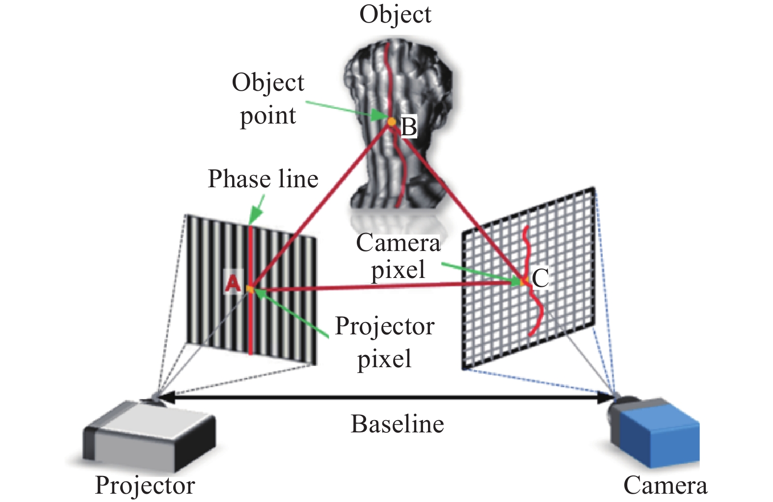
Fig. 1. Diagram of fringe projection 3D imaging
![Flowchart of phase calculation from a single fringe image using deep neural network[40]](/richHtml/irla/2020/49/3/0303018/img_2.jpg)
Fig. 2. Flowchart of phase calculation from a single fringe image using deep neural network[40]
Fig. 3. Comparison of 3D reconstruction results[40]. (a) Fourier transform profilometry, (b) windowed Fourier transform profilometry, (c) fringe analysis based on deep learning, and (d) 12-step phase-shifting profilometry
Fig. 4. Flowchart of label enhanced and patch based deep learning fringe analysis for phase retrieval[41]
Fig. 5. Phase measurement of hand movement at six different moments by FT and DNN methods[41]
Fig. 6. Diagram of fringe image denoising using deep learning[42]
Fig. 7. Test results[42]. (a1), (a2) Simulation fringe pattern with noise; (b1), (b2) fringe pattern without noise; (c1), (c2) denoised results with deep learning
Fig. 8. Schematic of phase unwrapping using PhaseNet[43]
Fig. 9. Results of different wrapped shapes using PhaseNet[43]. (a) Wrapped phase; (b) unwrapped phase; (c) fringe order with PhaseNet
Fig. 10. Schematics of the training and testing of the neural network[44]. (a) training; (b) testing
Fig. 11. Comparison of results of phase unwrapping of dynamic candle flame[44]. Wrap represents the wrapped phase; CNN represents the phase unwrapped by this method; LS represents the phase unwrapped by the least square method; Diff represents the difference between the results of CNN and LS methods
Fig. 12. Schematic of temporal phase unwrapping using deep learning[45]
Fig. 13. Comparison between traditional MF-TPU and the deep learning based method for high-frequency phase unwrapping (for example, the frequencies are 8, 16, 32, 48 and 64 respectively) [45]
Fig. 14. Neural network structure diagram of height estimation from a single fringe image[46]
Fig. 15. Experimental results of spherical, triangular bevel and face image grating[46]. The first column is the fringe image of the input neural network; the second column is the true simulated height distribution; the third column is the height distribution of the output of the neural network; the last column is the error distribution map based on the second column and the third column
Fig. 16. Flowchart for projector distortion correction with deep learning[47]
Fig. 17. Test results[47]. (a) 3D shape of the original data; (b) error distribution of the original data; (c) 3D shape of the corrected data; (d) error distribution of the corrected data
Fig. 18. Diagram of micro deep learning profilometry[49]
Fig. 19. High speed 3D imaging of a falling table tennis and static plaster at speed of 20 000 frame/s[49]


Set citation alerts for the article
Please enter your email address

© Copyright 2018-2021 | Chinese Laser Press. All Rights Reserved 沪ICP备15018463号-20