Statistical dynamics of noise-like rectangle pulse fiber laser

Yujia Li; Dongmei Huang; Yihuan Shi; Chao Wang; Feng Li

doi:10.1117/1.APN.2.3.036005

Abstract

The statistical dynamics of partially incoherent ultrafast lasers are complex and chaotic, which is significant for fundamental research and practical applications. We experimentally and theoretically reveal the statistical dynamics of the spectral evolutions and correlations in an incoherent noise-like rectangle pulse laser (NLRPL). Based on statistical histogram analysis, the probability distribution asymmetry of the spectral intensity fluctuation is decayed with the wavelength far away from the spectral peak due to the detection noise. The full-spectral correlation values indicate that the spectral similarity between two round trips is exponentially weakened as the round-trip offset increases. By studying the correlation map of spectral components, we find that the area of the high-correlation region is relevant to the pump power, which is reduced by increasing the pump power. The mutual information of the spectra demonstrates that two spectral components with symmetry about the spectral peak have a statistical dependence. Experimental observations and statistical properties can coincide well with theoretical numerical simulations. We reveal the pump-dependent spectral correlation of the NLRPL and provide multiple statistical methods for the characterizations of chaotic dynamics in incoherent light sources.

Keywords

fiber laser laser dynamics noise-like rectangle laser statistical analysis

1 Introduction

The noise-like pulse laser has complex and chaotic behaviors with random variable time durations and amplitudes, which has attracted great interest in the investigation, especially for ultrafast nonlinear optical physics.1^–4 The noise-like rectangle pulse laser (NLRPL) is one special case in the partially mode-locking operation region, whose duration of the pulse envelope can be flexibly tuned from picosecond to nanosecond order by changing the pump power while the pulse peak remains almost unchanged. Thus, NLRPL can easily obtain large pulse energy in a long cavity, which is promising in laser processing and micromachines.5 It can also be used to generate a supercontinuum (SC) source.6^,7 Noise-like pulse-pumped SC with low coherence and ultrawideband has been successfully employed in high-resolution spectral domain optical coherence tomography imaging.8 The fine spectral structure in the single-shot spectrum of the noise-like pulse is important to achieve a high-resolution location in distance metrology.9 Therefore, the generation mechanism and the application of noise-like pulse have been widely studied. Although the unique operation properties of the NLRPL, including the temporal versatile pattern dynamics and comparison with the dissipative soliton resonance have been presented,10^,11 the statistical dynamics in the fine spectral structure of the NLRPL still lack comprehensive experimental and theoretical explorations.

Dispersive Fourier transform (DFT) technology can realize single-shot spectral measurements using the huge group velocity dispersion (GVD) for time–frequency domain mapping.12^,13 It should be noted that DFT technology can continuously record large ensembles of single-shot spectra, making it possible to map the two-dimensional (2D) image of the spectral evolutions of the laser. This opens new opportunities for the characterization of abundant nonrepetitive phenomena in various ultrafast lasers, such as soliton-building dynamics,14^,15 soliton breathing,16^,17 soliton molecules,18^,19 optical rogue waves (ORWs),20^,21 and conventional noise-like pulses.22 Single-shot measurements of multiple round trips enable the statistical study of laser dynamics and nonlinear optics. One of the most typical statistical methods is the probability distribution of the spectral intensity fluctuation calculated from the statistical histogram, which has been used to reveal the ORW in nonlinear dissipative systems.20 Researchers analyzed the properties of the Raman ORW in a partially mode-locked Yb-doped fiber laser by combining the DFT with the histogram method.23 In addition, the pulse peak power for the noise-like pulse generation in a partial mode-locked laser has also been statistically revealed with a Gaussian distribution.2 The statistical histogram of energies of noise-like pulsing at subnanosecond scale in a passively mode-locked fiber laser shows that the subpulses are distributed to three primary discrete levels with a quantized nature, which is an exciting and fundamental finding benefiting from probability distribution analysis.24 However, the probability distribution of the spectral intensity fluctuations in the NLRPL still lacks experimental studies, which will be revealed by the statistical histogram in this work.

The spectral correlation provides another important analysis for the characterization of statistical dynamics for the partially coherent or incoherent light sources. Especially used as a pump for SC generation, the spectral correlation of the seed NLRPL will influence the spectral stability and coherence of the SC. Full spectral correlation or localized spectral correlation methods have been proposed to study the similarities or intensity distribution of the spectral components. Full spectral correlation values have been demonstrated to estimate the similarities of spectral behaviors between bidirectional solitons in the bidirectional mode-locked fiber, 17^,25 which loses the localized spectral details in different round trips. The Pearson correlation coefficient, as one crucial statistical parameter, has been used to analyze the localized spectral correlation in partially coherent light sources.26^,27 It has been successfully utilized to reveal the correlation of the intensity fluctuation between the two spectral components in the randomly distributed feedback fiber laser28 and the SC.29 However, the Pearson coefficient can only analyze the linear dependence of the spectral intensity fluctuation. Mutual information (MI), as another statistical tool, can measure both connotative linear and nonlinear dependences between two variables.30 It was proposed as a statistic concept in the field of information theory, which has been widely used to analyze the chaotic dynamics of nonlinear processes in optical fiber communication and artificial intelligence.31^,32 Recently, it has been utilized to successfully reveal the spectral correlation in the random fiber laser,29 instability beyond stable mode locking,33 and the optical parametric fiber oscillator.34 The NLRPL contains random and complex spectral information if we analyze it from a single spectral component. Its spectral components have controllable statistical properties, which will be revealed by studying the full spectral correlation values, Pearson coefficient, and MI in this work.

Sign up for Advanced Photonics Nexus TOC. Get the latest issue of Advanced Photonics Nexus delivered right to you！Sign up now

In this work, the fine spectral statistical dynamics of the NLRPL are fully characterized and analyzed in the experiment and theoretical simulation. The NLRPL is generated from a passively mode-locked fiber laser cavity based on a semiconductor saturable absorption mirror (SESAM). The single-shot spectra of the NLRPL are captured by the DFT spectroscope, which will provide the database of the statistical analysis. The probability distribution of the intensity jitters of full spectra and localized spectral components are studied by the statistical histogram. The shape of the probability distribution at different spectral components has an asymmetry that will be weakened with the wavelength far away from the spectral center. Then, the full-spectral correlation value, Pearson coefficient, and MI are used to analyze the spectral evolution dynamics of the NLRPL. The good match between the experimental analysis based on large sets of data and theoretical calculation based on the classical numerical model further confirms the validity and universality of the statistical dynamics. These results successfully reveal the statistical dynamics from the distorted single-shot spectral evolution, such as the exponential decaying of the spectral similarity and the pump-power-relevant localized spectral correlations. When used as the pump to generate the SC source, the spectral correlation of the SC is relevant to that of the NLRPL. Our findings by statistical analysis are significant in understanding the instabilities and randomness of other low-coherent light sources with chaotic and random behavior.

2 Experimental Setup

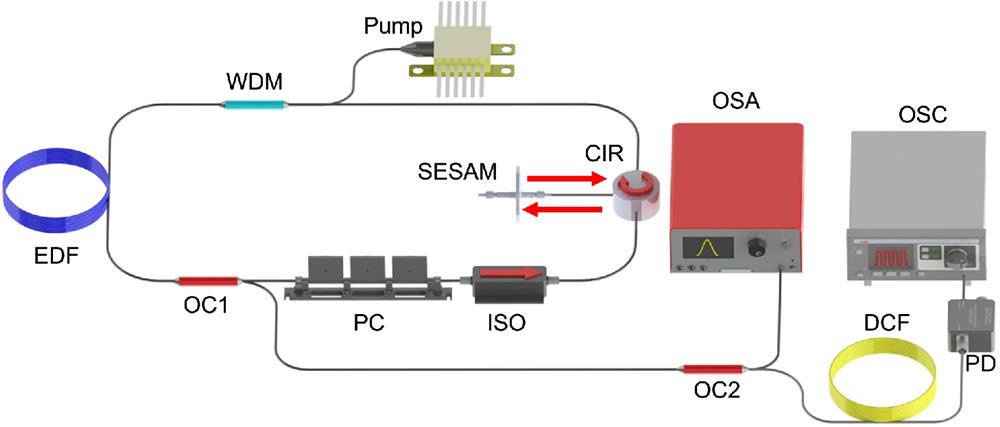
The experimental setup is shown in Fig. 1. The gain is provided by a piece of 2-m erbium-doped fiber (EDF, Er30-4/125, Liekki) with GVD of $+ 14.45 {ps}^{2} / km$ . The EDF is pumped by a 1480-nm continuous wave laser with a 1480/1550 wavelength division multiplexer (WDM). The isolator (ISO) ensures the laser’s one-way operation and avoids backreflecting light outside the cavity. A 90:10 optical coupler provides 90% of the light propagating inside the cavity and 10% of the light as the output. A commercial SESAM (SAM-1550-33-2ps, BATOP) is the saturable absorber to achieve mode locking, which is connected to port 2 of the optical circulator (CIR). The reflected light of the SESAM will enter the cavity through port 3 of the optical circulator. The total cavity length is about 16.3 m, containing the standard single-mode fiber with an effective length of about 14.3 m (double length for the two ports of the CIR). The average spectra of the output laser are measured by an optical spectrum analyzer (OSA, AQ6370D, YOKOGAWA) with a minimum resolution of 0.05 nm. We use two cascaded dispersion compensation fiber (DCF) modules with net effective group delay dispersion (DL) of $2506.3 ps / nm$ to obtain the single-shot spectrum in the DFT characterization. The stretched pulse after the DCF modules is detected by a high-speed photodetector (PD, BPDV2150R, Finisar) with a bandwidth of 43 GHz and a real-time high-speed oscilloscope (OSC, DSA-X, 96204Q, Agilent). The selected detection bandwidth and the sampling rate of the oscilloscope are 33 GHz ( $Δ ν$ ) and $80 GS / s$ , respectively. Thus, the obtained spectral resolution of the DFT characterization is about 0.012 nm, which can be simply estimated by $Δ λ = 1 / (DL Δ ν)$ .35

Figure 1.Experimental setup of the mode-locked fiber laser and characterization system of the spectrum. EDF, erbium-doped fiber; WDM, wavelength division multiplexer; ISO, isolator; OC, optical coupler; PC, polarization controller; CIR, circulator; SESAM, semiconductor saturable absorption mirror; DCF, dispersion compensation fiber; OSA, optical spectrum analyzer; OSC, oscilloscope.

3 Experimental Results and Discussion

3.1 Spectral Evolution

The basic operation properties, including the output spectrum, temporal pulse train, radio frequency (RF) spectrum, and the autocorrection trace of the NLRPL, are shown in Fig. S1 in the Supplemental Material. The DFT technology is used to observe the evolution of the single-shot spectra. We compare the average spectra obtained by the OSA and the DFT under the pump powers of 49, 135, and 365 mW (shown in Fig. S2 in the Supplemental Material), which indicates that the DFT characterization can acquire the correct single-shot spectra. The one-dimensional (1D) plots of the corresponding single-shot spectra are shown in Fig. S3 in the Supplemental Material. The 2D spectral map with the pump power of 49 mW within 4000 round trips is shown in Fig. 2(a). Unlike a highly coherent mode-locking state, the spectral evolution of the NLRPL is random. Therefore, the single-shot spectrum varies dramatically in different round trips. As a result, we can observe many spectral spots with irregular shapes in the 2D maps, where the region inside the white circle is a typical example. The spectral evolutions and the irregular spectral spots are relevant to the pump power, as shown in Figs. 2(b) and 2(c), with 135 and 365 mW, where the spectral spots become smaller with the enhancement of the pump power. The corresponding evolutions of the pulse envelopes with different pump powers are shown in Figs. 2(d)–2(f), where the width of the pulse envelope is widened as the pump power increases. Due to the limited bandwidth of the PD, we can hardly observe the noise-like pulse cluster under the rectangular envelope, which will be further studied in the numerical simulation. Here, the spectral evolution of the NLPRL under different pump powers can scarcely represent the accessible spectral dynamics due to the disorganized jitter of the spectral intensity. Thus, the quantitative relationship between the pulse envelopes and the single-shot spectra is missing, which will be statistically analyzed in the following contents.

Figure 2.Spectral and pulse-envelope evolutions within 4000 round trips. (a)–(c) Single-shot spectral evolution and (d)–(f) pulse envelope evolution of the NLRPL with the pump powers of 49, 135, and 365 mW, respectively.

3.2 Statistical Histogram of the Spectral Fluctuation

Both the spectral peak and energy are continuously recorded to study the spectral and pulse dynamics of the NLPRL, as shown in Fig. 3 in the 2D map. Figure 3(a) shows the three-dimensional scatter diagram of the normalized spectral energy and peaks with the pump power of 414 mW in 4000 round trips. The corresponding single-shot spectral evolution is shown in Fig. S4(a) in the Supplemental Material. We can see that the distribution of the scatters generates an elliptic region, and the relationship of the spectral energy and peak cannot be fitted by a particular analytic function. (The jitters of the spectral energy and peak in the time domain are shown in Figs. S4(b) and S4(d) in the Supplemental Material.) To further study the detailed statistical properties of the spectral dynamics, we use the histogram to represent the probability distribution of the spectral energy and peak. Figure 3(b) shows the joint probability distribution of the spectral energy and peak of 251,660 round trips. The distribution range of the spectral peak is larger than that of spectral energy. The spectral energy has a symmetrical Gaussian distribution shape with respect to the vertical dashed line (the marginal probability distribution of the spectral energy is shown in Fig. S4(c) in the Supplemental Material). Unlike the spectral energy, the spectral peak represents an asymmetrical long-tailed statistical distribution (the marginal probability distribution of the spectral peak is shown in Fig. S4(e) in the Supplemental Material). Therefore, there may exist a probability of generating rare wave events with giant amplitude. The significant wave height (SWH) based on the amplitude of the spectral peaks is calculated, which is defined as the mean amplitude of the highest third of the spectral peaks.21 The calculated SWH is 0.6231 (normalized maximum peak intensity is 1), indicating that the ORW is not generated in the NLRPL state.

Figure 3.Statistical properties of the spectral energy and peak. (a) 3D scatter diagram and the top view of the normalized spectral energy and spectral peak within 4000 round trips; (b) joint probability distribution of the spectral energy and spectral peak; (c) power spectral density of the jitter of the normalized spectral energy and spectral peak.

To quantifiably study the instabilities of the spectral energy and peak, the jitter curves of these two parameters are obtained by calculating the power spectral density of the relative jitters, as shown in Fig. 3(c). The noise distribution is relatively flat, especially in the high-frequency region after 1 MHz, which means that the high-frequency energy jitter has a similar property as the white noise with Gaussian-like probability distribution. However, there is a broad noise peak on the black curve near the frequency offset of 100 kHz due to the low-frequency jitter of the spectral energy. The frequency peak position is almost positively related to the pump powers. The detailed studies of the noise peaks under different pump powers are shown in Fig. S5 in the Supplemental Material. The red curve in the high-frequency region declines in the frequency-offset region after 1 MHz, which coincides with the probability distribution with the Gaussian deviation shape.

The average spectrum of the NLRPL obtained by the DFT with 251,160 samples with a pump power of 414 mW is shown in Fig. 4(a). The spectral shape is symmetrically trigonal. To further study the detailed statistical properties of the spectral dynamics, we select five spectral components [the five dashed lines in Fig. 4(a)] to observe the statistical histogram of the spectral fluctuation, as shown in Figs. 4(i)–4(v), where Fig. 4(iii) aligns with the peak wavelength. These statistical histograms have an asymmetrical shape. To study the appeared huge spectral intensity with a rare probability, we refer to the same statistical method of the ORW to identify the extreme wave event of the intensity at different spectral components. When the wavelength channel is far away from the peak wavelength, the asymmetry is weak, and the relative intensity of SWH is 0.5324, as shown in Fig. 4(i). Thus, no extreme wave events are generated at these spectral components, as shown in Figs. 4(i) and 4(ii). With the wavelength approaching the peak wavelength, the asymmetry of the distribution shape is enhanced. In addition, the SWH decreases to 0.3164, as shown in Fig. 4(iii). The intensity is 2 times as large as the SWH (marked by the red dashed line), which can be regarded as an extreme wave event. The experimental results indicate that the spectral extreme wave event generates at this spectral component. The asymmetry is weakened when the wavelength is far away from the peak wavelength, as shown in Figs. 4(iv) and 4(v). The obtained probability distribution should contribute to the light fluctuation with the inherently asymmetrical probability distribution and the detection noise of the PD and OSC with the symmetrical distribution. Because the spectral intensity at two sides is weaker than that of the spectral center, the proportion of the noise induced by the PD will become larger with weaker light intensity. Since the probability distribution of this noise is highly symmetrical, the symmetry of the probability distribution of the intensity fluctuation is stronger when the spectral component is far away from the spectral center. When the calculated SWH increases to 0.5695 in Fig. 4(v), the spectral extreme wave event will completely disappear. The 2D map of the probability distribution of the normalized fluctuations at the spectral components with the wavelength from 1555 to 1563 nm is plotted to study the evolution of the statistical properties, as shown in Fig. 4(b). The probability distribution is obtained based on the statistical histogram. The asymmetry of the probability distribution at either end is obviously weaker than that at the wavelengths near the peak wavelength. The SHWs at different channels are calculated, as shown in Fig. 4(b). When the value of the SHW is $< 0.5$ , extreme wave events are generated for these spectral components, which are marked by the green region. We can calculate the probability of the spectral extreme wave events in all wavelength channels, as shown in Fig. 4(d). As the intensity increases from the spectral edge to the center, the generation probability of extreme wave events increases. The maximum probability of the extreme wave events is located at about 1558.23 nm, close to the peak wavelength, which is only about 0.58%. In this wavelength channel, the threshold intensity of the extreme wave event is about 0.5732, which is around 5 times the average intensity (0.1290). The related numerical simulation results are presented in the Supplemental Material.

Figure 4.Statistical properties of the spectral components with 251,160 round trips. (a) Average spectrum of the NLRPL obtained by 251,160 single-shot spectra; (i)–(v) statistical histograms of the intensity fluctuation at the spectral components of 1556.02, 1556.70, 1558.72, 1560.92, and 1561.81 nm, respectively. (b) 2D map of the probability distribution of the spectral fluctuations, (c) SHWs, and (d) generation probabilities of the extreme wave events at all spectral components corresponding to (a).

3.3 Spectral Correlation Analysis

Different from the coherent mode locking with stable operation, the NLRPL is partially mode-locked with random spectral evolution, which has been shown in Fig. 2. To quantifiably study the spectral behavior, the spectral similarity between arbitrarily two different round trips can be estimated by calculating the full spectral correlation values as25 $ξ (R_{j}, R_{i}) = \frac{{[\int I (λ, R_{i}) I (λ, R_{j}) d λ]}^{2}}{\int {[I (λ, R_{i})]}^{2} d λ \int {[I (λ, R_{j})]}^{2} d λ},$ (1)where $I (λ, R_{i})$ and $I (λ, R_{j})$ are the intensities at the spectral component of $λ$ in the $i$ th and $j$ th round trip, respectively, and $ξ (R_{i}, R_{j})$ is the spectral correlation value between the $i$ th and $j$ th round trip. If the spectra of two round trips are the same, the correlation value equals 1, and the higher spectral similarity makes the value closer to 1. The 2D map of the full spectral correlation values within 4000 round trips is shown in Fig. 5(a). The values near the 45-deg diagonal line are higher than those of the other region, which means that the two single-shot spectra are similar only when they are very close. When we fix the value of $i$ and change the value of $j$ , the 1D correlation curves are shown in Fig. 5(b), where $i = 1 + 20 (n - 1)$ ( $n = 1, 2, 3, \dots, 250$ ) and $j - I = 0,1 \dots, 50$ . The round-trip offset equals $j - i$ . The dashed line is the average result of the 250 curves, and the corresponding fitting curves by $y = a e^{- b x} + c$ have an $R^{2}$ of 0.9920, where $a$ , $b$ , and $c$ equal 0.386, 0.2721, and 0.6291, respectively. The parameter $b^{- 1}$ is negatively related to the decay speed of the spectral similarity. The correlation values exponentially decrease by increasing the round-trip offset. The correlation curves within the offset number from 51 to 10,000 are shown in the inset of Fig. 5(b) ( $i = 1, j - i = 51, 52, \dots, 10,000$ ), where the correlation value will not be continuously decayed and finally varies around a constant. The fitting values of $b^{- 1}$ under different pump powers are shown in Fig. 5(c), where the values will decrease as the pump power increases. (The results of the full spectral correlation analysis under other pump powers are provided in Fig. S6 in the Supplemental Material.) When the pump power is lower, the spectral evolution map contains larger spots and more obvious continuity. The spectral similarity has a slower decay. In this case, the turbulence degree of the spectral evolution process is lower than the situations with higher pump powers, resulting in the decrement of $b^{- 1}$ . The full spectral correlation analysis successfully reveals the dynamics of the spectral similarity decay from the distorted evolution maps.

Figure 5.Analysis results based on the full spectral correlation values. (a) 2D map of the full spectral correlation values within 4000 round trips; (b) spectral correlation curves within the total round-trip offset number of 50; the inset is the spectral correlation curve with the round-trip offset number from 51 to 4000; (c) fitted $b^{- 1}$ values of the correlation curve under different values.

The full spectral correlation analysis cannot present the statistical performance of the localized spectra. The correlations of the localized spectral components can be revealed by calculating the Pearson coefficient, which statistically represents the linear correlation of the shot-to-shot fluctuations of the intensity at two arbitrary wavelengths.24 The intensity at the wavelength channel of $λ_{x}$ of the $i$ th round trip is defined as $I (λ_{x}, T_{i})$ , which can be obtained by the DFT technology. The Pearson correlation coefficient between the two wavelengths $λ_{x}$ and $λ_{y}$ can be expressed as27 $ρ (λ_{x}, λ_{y}) = \frac{\frac{1}{N} \sum_{i = 1}^{N} I (λ_{x}, T_{i}) I (λ_{y}, T_{i}) - \frac{1}{N^{2}} \sum_{i = 1}^{N} I (λ_{x}, T_{i}) \sum_{i = 1}^{N} I (λ_{y}, T_{i})}{\sqrt{\frac{1}{N} \sum_{i = 1}^{N} I^{2} (λ_{x}, T_{i}) - \frac{1}{N^{2}} {[\sum_{i = 1}^{N} I (λ_{x}, T_{i})]}^{2} \sqrt{\frac{1}{N} \sum_{i = 1}^{N} I^{2} (λ_{y}, T_{i}) - \frac{1}{N^{2}} {[\sum_{i = 1}^{N} I (λ_{y}, T_{i})]}^{2}}}},$ (2)where $N$ is the total number of the round trips. The value of the Pearson coefficient only varies from $- 1$ to 1. When the Pearson coefficient is positive (negative), $I (λ_{x})$ and $I (λ_{y})$ are positively (negatively) correlated. The absolute value of the Pearson coefficient is larger, and the linear correlation of the two variables will be higher. If two variables $I (λ_{x})$ and $I (λ_{y})$ have a particular linear relationship, the amplitude of $ρ (λ_{x}, λ_{y})$ equals 1. If two variables are mutually independent, the amplitude of $ρ (λ_{x}, λ_{y})$ equals 0. Using Eq. (2), we can obtain the spectral correlation maps by calculating the absolute value of the Pearson coefficient based on the spectral evolution within 4000 continuous round trips, as shown in Fig. 6.

Figure 6.Analysis results based on the Pearson correlation coefficient with 4000 round trips. (a)–(c) Spectral correlation maps based on the absolute value of the Pearson correlation coefficient; (d) corresponding spectral correlation curves crossing the peak wavelength with the pump powers of 49, 135, and 365 mW; (e), (f) FWHMs of the spectral correlation curves, the productions of the FWHMs (with the unit of hertz), and the pulse widths under different pump powers.

Figures 6(a)–6(c) show the spectral correlation maps within the wavelength range from 1558 to 1560 nm under the pump power of 49, 135, and 365 mW, respectively. As shown in Fig. 6(a), the values near the diagonal line are larger than those in another region, which means that the shot-to-shot intensity fluctuation at a particular wavelength is only linearly correlated to that at the neighboring wavelengths. This blue region means that the intensity fluctuation at two far-away wavelengths is almost independent. As shown in Figs. 6(b) and 6(c), the area of the red region is reduced by increasing the pump power. We can see that the spectrum of the NLRPL just has a localized high correlation. To demonstrate the relationship between the spectral correlation and pump power, we plot the 1D dashed cutting lines [Fig. 6(c)] of these maps passing through the peak wavelength, as shown in Fig. 6(d). Through increasing the pump power, the full width at half-maximum (FWHM) of the spectral correlation curves is narrowed. The FWHMs with different pump powers from 49 to 414 mW are shown in Fig. 6(e), which vary from 0.132 to 0.014 nm. The FWHM of the 1D cutting lines crossing through the wavelengths in the range from $peak - δ$ to $peak + δ$ is calculated ( $δ \approx 1 nm$ ). The error bars are obtained by calculating the corresponding standard deviation. The FWHM monotonously decreases, and the change rate of the FWHW also slows down. It should be noted that the FWHM is much narrower than the whole spectral energy range, indicating that there is only a high correlation within the localized spectral region. Then, we plot the corresponding pulse of the NLRPL in the time domain. Similar to the previous studies, the pulse duration is linearly broadened from 52.2 to 591.7 ps, with the pump power increasing from 49 to 414 mW. The corresponding average pulse envelopes with different pump powers are provided in Fig. S7 in the Supplemental Material. We also further study the production of the pulse width and the FWHM under different pump powers, as shown in Fig. 6(f). Though the pulse is broadened by 1 order, the value of the production just slightly varies from 0.815 to 1.009. Thus, the FWHM of the NLRPL is almost inversely proportional to the duration of the pulse, indicating that the pump power can influence the spectral region with a high correlation.

As we know, the spectral correlation map can only represent the linear dependence of two random variables. In information theory, MI is the “amount of information” obtained through observing the other random variable after receiving the information of one random variable. Therefore, MI can precisely study the mutual nonlinear dependence and the difference in the probability distribution of two random variables. MI has been applied to characterize laser instabilities beyond a stable mode-locking operation.31 The MI of the shot-shot spectral fluctuation in two spectral components can be expressed by $MI (λ_{x}, λ_{y}) = H (λ_{x}) + H (λ_{y}) - H (λ_{x}, λ_{y})$ , where $H (λ_{x})$ and $H (λ_{y})$ are the Shannon entropy of $I (λ_{x})$ and $I (λ_{y})$ , respectively, and $H (λ_{x}, λ_{y})$ are the joint entropy of $I (λ_{x})$ and $I (λ_{y})$ . Their joint probability distributions are calculated to represent the statistical dependence between the peak wavelength and another wavelength, as shown in Figs. 7(a)–7(c). The wavelength intervals are 0.015, 0.01, and 0.005 nm, and the statistical sample number is 251,160. The shapes of the joint probability distributions are simultaneously dispersed toward the larger spectral intensity. The two red lines generate a divergence angle of the distribution shape, which can intuitively represent the total dependence between the two wavelengths. By decreasing the wavelength interval, the angle of divergence becomes smaller while the normalized MI value becomes larger, indicating an enhanced statistical dependence.

Figure 7.Analysis results based on the MI. (a)–(c) Joint probability distributions and the normalized MI values of the spectral intensities between the peak wavelength (1558.72 nm) and the wavelength with intervals of 0.015, 0.01, and 0.005 nm, respectively (251,160 round trips); (d) 2D map of the normalized MI of two arbitrary wavelengths within the range from 1556 to 1562 nm, which is obtained by the spectral evolution with continuous 4000 round trips; (e) normalized MI values on the blue 1D cutting line in (d) with different total round trips; (f) average values of MI within the black shadow region with different total round trips.

The 2D map with the normalized MI values between two arbitrary wavelengths within the range from 1555 to 1563 nm is shown in Fig. 7(d). The normalized MI values, $MI (λ_{x}, λ_{y})$ , at the rising diagonal line always equal 1, since $λ_{x}$ equals $λ_{y}$ . Due to the reciprocity $[MI (λ_{x}, λ_{y}) = MI (λ_{y}, λ_{x})]$ , the 2D map has symmetry with respect to the rising diagonal line. However, except for the rising diagonal line, the MI map is almost symmetrical with respect to the other three dashed lines. The intersection of these lines is close to the peak wavelength point $(λ_{x}, λ_{y})$ , where both $λ_{x}$ and $λ_{y}$ equal 1558.72 nm. The spectral fluctuation of one wavelength does not only have a dependence on that of the spectral component with a small wavelength interval, but it is also highly correlated to the symmetrical peak wavelength [for example, point A (1560.42 nm, 1560.36 nm, 0.2054) and point B (1560.42 nm, 1557.08 nm, 0.2337)]. From the results in Fig. 7(d), we can predict that the statistical property of the spectral fluctuation has symmetry about the spectral center. To observe the change of normalized MI with large different wavelength intervals, the normalized MI values on the blue dashed cutting line under different wavelengths are plotted in Fig. 7(e), and the wavelength resolution of the curve is $\sim 0.025 nm$ . With the increment of the statistical round-trip number, no wavelength shift of the peak is observed. The normalized MI curve integrally decreases with the symmetrical shape. The average values of MI with different round trips are shown in Fig. 7(f), which are obtained by calculating the average value of the normalized MI curve in the shadow region with a wavelength range of $\sim 0.5 nm$ (except for the peak value of 1), as shown in Fig. 7(e). The error bar is obtained by calculating the corresponding standard deviation. The decline rate of the normalized MI becomes slower and finally converges to almost 0. This means that the uncertainty of the intensity fluctuation at two wavelengths is gradually weakened with the increment of the total round trips. Further increasing the round trips for two different wavelengths, the statistical certainty and coherence will be totally lost.

4 Numerical Simulations

To verify whether the observed dynamics of the NLRPL are general, we use numerical simulations of the laser according to the complex Ginzburg-–Landau equation, which can be expressed as36 $\frac{\partial A}{\partial z} = - i \frac{β_{2}}{2} \frac{\partial^{2} A}{\partial T^{2}} + i γ {| A |}^{2} A + \frac{g - α}{2} A + \frac{g}{2 Ω_{g}^{2}} \frac{\partial^{2} A}{\partial T^{2}},$ (3)where $β_{2}$ is the GVD, $γ$ is the nonlinear coefficient, $α$ is the fiber loss (=0.2 dB/km), and $Ω_{g}$ is the gain bandwidth (6.245 THz) of the EDF. $g$ is the gain of the EDF, which is determined by $g = g_{0} \exp (- E_{p} / E_{s})$ . $g_{0} = 4 m^{- 1}$ is defined as the small signal gain of the EDF. $E_{p}$ is the pulse energy, and $E_{s}$ is the saturable pulse energy of the EDF. In the simulation, the total lengths of the EDF and SMF are 2 and 14.3 m, respectively. The GVDs of the SMF and EDF are $- 21.7$ and $14.45 {ps}^{2} / km$ , and the nonlinear coefficients of the SMF and EDF are 1.3 and $2.8 W^{- 1} {km}^{- 1}$ , respectively. We ignore the recovery time of the saturable absorber in the simulation, and the transmission of the saturable absorber can be simply expressed by $T (P) = 1 - α_{0} - α_{n} / (1 + P / P_{s})$ , where $α_{0} = 0.14$ and $α_{n} = 0.19$ are the linear and nonlinear absorption coefficients, respectively. $P_{s} = 240 W$ is the saturable power of the saturable absorber. When we set the EDF’s saturable pulse energy $E_{s}$ as 1.2 nJ, the laser can operate in the NLRPL state. We would like to point out that all the parameters in the simulation are approximate to the experiment but not completely the same. The inner cavity evolutions, including the single-shot spectrum, intensity in the time domain, and pulse energy are shown in Fig. S8 in the Supplemental Material. As shown in Figs. 8(a)–8(c), similar to the experimental results, the spectral behaviors are very random and disorganized in the NLRPL state. The change of the single-shot spectral evolutions with the pump power enhanced matches the experimental results in Figs. 2(a)–2(c), where the spectral spots will become smaller. The corresponding pulse evolutions in the time- domain under different saturable energies are shown in Figs. 8(d)–8(f). We can obtain the random internal movements of the pulse cluster. With the saturable pulse energy enhanced, the distribution range of the pulse is widened. However, due to the limited bandwidth of the PD, only a rectangle-like pulse envelope is experimentally observed, coinciding with the results in Fig. S7 in the Supplemental Material.

Figure 8.Numerical simulation results of the spectrum and pulse-envelope evolutions (4000 round trips). (a)–(c) Single-shot spectral evolution and (d)–(f) pulse envelope evolution of the NLRPL with the saturable pulse energies of 0.2, 0.4, and 1.2 nJ, respectively.

The simulated intensity autocorrelation trace of the NLRPL is also studied and presented in Fig. 9(a). A typical strong coherence peak matches well with the experimental results in Fig. S1(d) in the Supplemental Material. The 2D wavelength-time spectrogram is calculated by the short-time Fourier transform,37 as shown in Fig. 9(b). The time window of the Fourier transform is 7.8 ps, corresponding to a spectral resolution of about 1 nm. There are interference patterns on the short-time spectrogram due to the interaction between multiple pulses within the time window. Since the pulse numbers within most time windows are $< 3$ , the spectral pattern has a periodical distribution that is similar to the soliton molecule’s spectral interference.19 The blue curve is the spectrum of the total time window of 2 ns, which are the synthetical results of mutual interferences of all pulses with random phases and intervals (shown as the black curve). The pulses of the simulated NLRPLs with different saturable energies are shown in Fig. 9(c), which are obtained by calculating the average trace of 9000 single-shot pulse traces in the time domain. The pulse width gradually broadens by increasing the saturable energy. The pulse features further verify that our numerical simulations match well with the experimental results, which can provide qualitative guidance for us to further statistically study the NLRPL, including the spectral evolutions and spectral coherence.

Figure 9.Numerical simulation results of NLRPL. (a) Intensity autocorrelation trace; (b) 2D wavelength-time spectrogram and the corresponding intensity in time domain and spectrum. (c) Pulse envelopes under different saturable energies; (d)–(f) spectral correlation maps based on the absolute value of the Pearson correlation coefficient (4000 round trips); (g) corresponding spectral correlation curves crossing the peak wavelength with the saturable energies of 0.2, 0.4, and 1.2 nJ; (h), (i) FWHMs of the spectral correlation curves and the productions of the FWHMs (with the unit of hertz) and the pulse widths under different saturable energies.

Similar to Fig. 6, the 2D map of the Pearson correlation coefficient is also calculated through the simulated spectral evolution, as shown in Figs. 9(d)–9(f). By increasing the saturable energy, the area of the red region with a higher Pearson correlation coefficient decreases, which coincides well with the experimental results. Then, we calculated the FWHM of the coefficient curve, and the values with different pump powers are shown in Fig. 9(h), where the FWHM narrows from 0.077 to 0.0136 nm by increasing the saturable energy. The corresponding pulse width varies from 82.7 to 524 ps. To conveniently estimate the pulse width, the average pulse envelope is smoothed by a window of 100 points. The pulse width is obtained by calculating the pulse width with an intensity that is higher than 20% of the pulse peak. As shown in Fig. 9(i), the production of the FWHM and pulse width vary slightly within the range from 0.79 to 0.93, which is similar to the experimental results. More detailed statistical dynamics obtained by the numerical simulations are shown in Figs. S9 and S10 in the Supplemental Material. These simulation results, such as the statistical properties of the spectral energy and peak, statistical properties of the spectral components, and analysis results based on the MI, can be coincided well with the experimental results in Figs. 3, 4, and 7, respectively.

One important application of the noise-like pulse is to stimulate the SC. The spectral Pearson correlation coefficient provides a method to statistically characterize the spectral instability and coherence of the SC, which is critical in evaluating the dynamical performance of the SC. Here, we theoretically study the spectral correlation of the SC pumped by the NLRPL pulse using the generalized nonlinear Schrödinger equation. 38 The simulation model and parameters for the simulation are shown in Eq. (S2) and Table S1 in the Supplemental Material. The detailed spectral evolutions of the generation of the SC pumped by the NLRPL and ${sech}^{2}$ pulse are shown in Fig. S11 in the Supplemental Material. In some practical applications, we care about the properties of the average spectra. Figure 10(a) shows the spectrum of the SC pumped by the ${sech}^{2}$ pulse. The ${sech}^{2}$ pulse is usually generated in the mode-locked laser outputting the conventional soliton. The pump pulse train is periodical. The generated SC is also theoretically periodical. Thus, the average spectrum of the SC should also coincide with the single-shot spectrum. Then, we use the SCs simulated by the NLRPL within continuous 1500 round trips to obtain the average spectra, as shown in Fig. 10(b). The black and brown curves are the single-shot and average spectra, respectively. The spectrum of the NLRPL varies round trip by round trip, and the generated SC also varies. Compared with the SC pump by the ${sech}^{2}$ pulse, though the spectral quality and coherence of the single-shot spectral of the NLRPL-pumped SC are poor, the average spectra have a flatter envelope. The flat and broadband spectrum is significant when it is applied in the spectral analysis and spectral-domain optical coherence tomography (OCT).

Figure 10.Numerical simulation results of the statistical dynamics of the SC and NLRPL. (a) 1D spectra of the SC pumped by the ${sech}^{2}$ pulse; (b) 1D single-shot and average spectra of the SC pumped by the NLRPL with the saturable energy of 1.2 nJ; (c)–(e) 2D Pearson coefficient maps of the SC pumped by the NLRPLs with the saturable energies of 0.2, 0.4, and 1.2 nJ, respectively. The wavelength range is marked by the red region in (b).

Then, we study the spectral correlations of the SC pumped by the NLRPL with different saturable energies. The widths of the high-correlation regions of the NLRPL will be narrowed by decreasing the saturable powers. This has been shown in Figs. 6 and 9. Figures 10(c)–10(e) show the spectral correlation maps based on the Pearson coefficient of the SC pumped by the corresponding NLRPLs. The wavelength range (from 1795 to 1798 nm) of the 2D maps is marked by the red region in Fig. 10(b). Obviously, the width of the high-correlation region for the SC is positively related to that of the pump laser (NLRPL). The above results indicate that the spectral statistical properties of the NLRPL will influence the spectral stability and coherence of the generated SC. Therefore, the spectral statistical dynamics of the NLRPL is important to help optimize the SC generation and its applications.

5 Conclusions

In this work, the spectral statistical dynamics, including the probability distributions and spectral correlations of the NLRPL, are studied with a DFT spectroscope. The intensity fluctuations’ probability distribution of the spectral component near the peak wavelength has an asymmetric shape and is weakened as the wavelength is far away from the peak wavelength. The probability distributions of the normalized intensity at different wavelengths indicate that the spectral extreme wave events are generated in the NLRPL. The correlation values of the full spectra demonstrate that the spectral similarity degrees between two round trips are exponentially weakened with the increase of round-trip offset, and the decay speed is positively related to the pump power. The Pearson correlation coefficients of the shot–spectral fluctuations at two arbitrary wavelengths reveal the localized spectral correlation of the NLRPL, and the correlation is relevant to the pump power. MI maps calculated from the Shannon entropy further confirm the statistical symmetry of the spectral intensity fluctuation with respect to the spectral center. These findings provide experimental and theoretical insight into the spectral correlation and statistical symmetry of NLRPL and further deepen our understanding of the random behaviors in the stochastically driven nonlinear optics.

Yujia Li received his BSc and PhD degrees from Chongqing University, Chongqing, China, in 2015 and 2020. He is currently a postdoc at the Photonics Research Institute of the Hong Kong Polytechnic University. His current research interests mainly include fiber lasers, laser dynamics, laser imaging, and nonlinear fiber optics.

Dongmei Huang received her BSc degree from Huazhong University of Science and Technology in 2014, her MSc degree from Chongqing University in 2017, and her PhD from the Hong Kong Polytechnic University, Kowloon, Hong Kong, in 2020. She is currently a research assistant professor at the Photonics Research Institute of the Hong Kong Polytechnic University. Her research interests include wavelength swept lasers and their applications in optical coherence tomography and optical sensing systems and nonlinear microresonators.

Yihuan Shi received his BSc and ME degrees from Northwest University, Xi’an, China, and Shenzhen University, Shenzhen, China, respectively. He is currently a PhD student at the Photonics Research Institute of the Hong Kong Polytechnic University. His current research interests mainly include Fourier domain mode-locked fiber lasers, optical coherence tomography, and nonlinear optics.

Chao Wang received his BSc degree from Huazhong University of Science and Technology, and his PhD from the East China Normal University, China, in 2013 and 2018, respectively. After that, in 2021, he was a postdoctoral fellow at the Hong Kong Polytechnic University, Kowloon, Hong Kong. His research interests include microwave photonics, ultrafast fiber lasers, dual-comb lasers, and their application in imaging, spectroscopy, and distance measurements.

Feng Li (member, IEEE; senior member, OSA) received his BSc and PhD degrees from the University of Science and Technology of China, Hefei, China, in 2001 and 2006, respectively. After that, he was a postdoctoral fellow at the Hong Kong Polytechnic University, Kowloon, Hong Kong. His research interests include fiber lasers, including mode-locked fiber lasers, multiwavelength fiber lasers, wavelength swept lasers and their application in biophotonics; nonlinear optics in optical fibers, microresonator/waveguides, including soliton propagation and supercontinuum generation; optoelectronic devices.

References

[1] A. F. J. Runge et al. Coherence and shot-to-shot spectral fluctuations in noise-like ultrafast fiber lasers. Opt. Lett., 38, 4327-4330(2013).

[2] Z. Wang et al. Q-switched-like soliton bunches and noise-like pulses generation in a partially mode-locked fiber laser. Opt. Express, 24, 14709-14716(2016).

[3] B. Li et al. Unveiling femtosecond rogue-wave structures in noise-like pulses by a stable and synchronized time magnifier. Opt. Lett., 44, 4351-4354(2019).

[4] R. Zhou et al. Quasi-coherent noise-like pulses in a mode-locked fiber laser with a 3D rotatable polarization beam splitter. Opt. Lett., 46, 1305-1308(2021).

[5] J. Liu et al. Generation and evolution of mode-locked noise-like square-wave pulses in a large-anomalous-dispersion Er-doped ring fiber laser. Opt. Express, 23, 6418-6427(2015).

[6] S. Lin, S. Hwang, J. Liu. Supercontinuum generation in highly nonlinear fibers using amplified noise-like optical pulses. Opt. Express, 22, 4152-4160(2014).

[7] H. Chen et al. Ultra-compact Watt-level flat supercontinuum source pumped by noise-like pulse from an all-fiber oscillator. Opt. Express, 23, 32909-32916(2015).

[8] Y. You et al. Ultrahigh-resolution optical coherence tomography at 1.3 μm central wavelength by using a supercontinuum source pumped by noise-like pulses. Laser Phys Lett., 13, 025101(2015).

[9] Y. Sun et al. Stretched noise-like pulse for high-resolution laser ranging, 1-2(2022).

[10] Y. Huang et al. Versatile patterns of multiple rectangular noiselike pulses in a fiber laser. Opt. Express, 24, 7356-7363(2016).

[11] K. Zhao et al. High-energy dissipative soliton resonance and rectangular noise-like pulse in a figure-9 Tm fiber laser. Appl. Phys. Express, 12, 012002(2019).