• Laser & Optoelectronics Progress
  • Vol. 57, Issue 22, 221011 (2020)
Bin Li1、* and Lu Ma2
Author Affiliations
  • 1Department of Basic Teaching, Suzhou Vocational and Technical College, Suzhou, Anhui 234099, China
  • 2Department of Computer Information, Suzhou Vocational and Technical College, Suzhou, Anhui 234099, China
  • show less
    DOI: 10.3788/LOP57.221011 Cite this Article Set citation alerts
    Bin Li, Lu Ma. Super-Resolution Reconstruction of Densely Connected Generative Adversarial Network Images[J]. Laser & Optoelectronics Progress, 2020, 57(22): 221011 Copy Citation Text show less
    Structure diagram of GANs
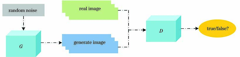
    Fig. 1. Structure diagram of GANs
    Generate network structure diagram
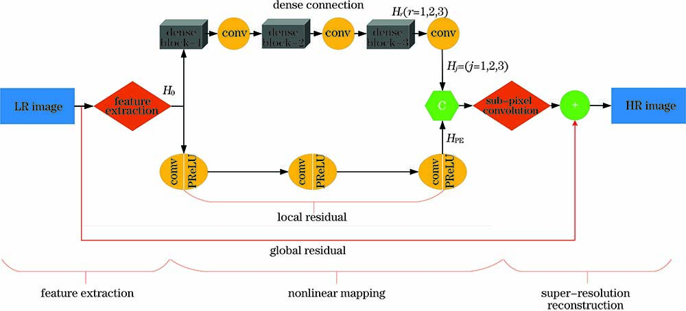
    Fig. 2. Generate network structure diagram
    Structure of densely connected blocks
    Fig. 3. Structure of densely connected blocks
    Discriminant network model
    Fig. 4. Discriminant network model
    Comparison of butterfly reconstruction effect. (a) Original image; (b)method in Ref. [23]; (c) method in Ref. [5]; (d) method in Ref. [7]; (e) method in Ref. [8]; (f) method in Ref. [13]; (g) method in Ref. [16]; (h)proposed method
    Fig. 5. Comparison of butterfly reconstruction effect. (a) Original image; (b)method in Ref. [23]; (c) method in Ref. [5]; (d) method in Ref. [7]; (e) method in Ref. [8]; (f) method in Ref. [13]; (g) method in Ref. [16]; (h)proposed method
    Comparison of lenna reconstruction effect. (a) Original image; (b)method in Ref. [23]; (c) method in Ref. [5]; (d) method in Ref. [7]; (e) method in Ref. [8]; (f) method in Ref. [13]; (g) method in Ref. [16]; (h)proposed method
    Fig. 6. Comparison of lenna reconstruction effect. (a) Original image; (b)method in Ref. [23]; (c) method in Ref. [5]; (d) method in Ref. [7]; (e) method in Ref. [8]; (f) method in Ref. [13]; (g) method in Ref. [16]; (h)proposed method
    Comparison of 253027 reconstruction effect. (a) Original image; (b)method in Ref. [23]; (c) method in Ref. [5]; (d) method in Ref. [7]; (e) method in Ref. [8]; (f) method in Ref. [13]; (g) method in Ref. [16]; (h)proposed method
    Fig. 7. Comparison of 253027 reconstruction effect. (a) Original image; (b)method in Ref. [23]; (c) method in Ref. [5]; (d) method in Ref. [7]; (e) method in Ref. [8]; (f) method in Ref. [13]; (g) method in Ref. [16]; (h)proposed method
    Comparison of barbara reconstruction effect. (a) Original image; (b)method in Ref. [23]; (c) method in Ref. [5]; (d) method in Ref. [7]; (e) method in Ref. [8]; (f) method in Ref. [13]; (g) method in Ref. [16]; (h)proposed method
    Fig. 8. Comparison of barbara reconstruction effect. (a) Original image; (b)method in Ref. [23]; (c) method in Ref. [5]; (d) method in Ref. [7]; (e) method in Ref. [8]; (f) method in Ref. [13]; (g) method in Ref. [16]; (h)proposed method
    Comparison of the number of parameters
    Fig. 9. Comparison of the number of parameters
    Comparison of image edge extraction before and after convolution operation. (a)--(c) Images after convolution operation; (d)--(f) corresponding images before convolution operation
    Fig. 10. Comparison of image edge extraction before and after convolution operation. (a)--(c) Images after convolution operation; (d)--(f) corresponding images before convolution operation
    DatasetScaleMethod inRef. [23]Method inRef. [5]Method inRef. [7]Method inRef.[8]Method inRef.[13]Method inRef. [16]Proposedmethod
    Set523433.5730.4229.0031.3936.6131.9930.2736.7232.8530.5637.4433.4531.1237.7133.9031.6237.9334.1131.79
    Set1423430.2427.5526.0028.3132.2829.1327.3232.4529.3027.5033.0329.7728.0133.2329.9228.1433.4430.0828.35
    B10023429.4927.1125.8827.8330.9728.1026.7931.4528.3826.9631.5728.9627.2231.9029.0127.3832.1329.3027.57
    Urban10023426.7624.5923.3025.3528.9426.0124.4529.4926.3324.6530.6927.2325.0930.8527.4425.3630.9727.5825.63
    Table 1. Comparison of PSNR between proposed algorithm and mainstream algorithm on four test sets unit:dB
    DatasetScaleMethod inRef. [23]Method inRef. [5]Method inRef. [7]Method inRef.[8]Method inRef.[13]Method inRef. [16]Proposedmethod
    Set52340.92930.86710.81150.88190.95000.90030.86220.95390.90880.86300.95760.92090.88390.95770.92280.88710.96030.92390.8877
    Set142340.86790.77380.70260.79370.90700.81770.74870.90570.82090.75210.91300.83250.76690.91310.83290.76780.91430.83260.7687
    B1002340.84290.73830.66800.74580.88540.78440.70690.88800.78570.71000.89550.79680.72470.89580.79810.72660.89930.79940.7280
    Urban1002340.84110.73380.65670.75540.89220.79080.71830.89510.79760.72330.91350.82660.75090.91500.82460.75370.91640.82990.7551
    Table 2. Comparison of SSIM between proposed algorithm and mainstream algorithm on four test sets
    DatasetScaleMethod inRef. [23]Method inRef. [5]Method inRef. [7]Method inRef.[8]Method inRef.[13]Method inRef. [16]Proposedmethod
    Set5234---0.470.580.320.242.192.232.190.130.140.120.210.190.220.110.130.12
    Set14234---0.510.840.560.384.324.404.390.250.260.250.270.230.210.220.210.20
    B100234---0.520.590.330.262.512.582.510.160.210.210.300.270.250.130.170.15
    Urban100234---0.692.961.671.2122.1219.3518.460.981.081.061.011.001.030.910.981.02
    Table 3. Comparison of time consumption between proposed algorithm and mainstream algorithms on four test sets unit:s
    Bin Li, Lu Ma. Super-Resolution Reconstruction of Densely Connected Generative Adversarial Network Images[J]. Laser & Optoelectronics Progress, 2020, 57(22): 221011
    Download Citation