Changes in land cover caused by land use have significantly altered the Earth in the late Quaternary (Kaplan et al., 2017). Long-term land use and land cover change (LUCC) is an important way to understand the processes of global and regional environment changes (Watson et al., 2000; Foley et al., 2005; Ellis et al., 2013; Zhang et al., 2019). Numerous scholars have therefore attempted to reconstruct past LUCC at different spatiotemporal scales (Li et al., 2018). Forests, as among the most widespread forms of land cover on Earth (Darby, 1956; Hughes and Thirgood, 1982), have played an important role in regulating climate, the surface radiation budget, and greenhouse gases (House et al., 2002; Werf et al., 2009). Thus, forest data over long time periods are essential to modeling global or regional climate changes and their ecological effects.

Considerable progress has been made in reconstructing historical forest cover at the local and global scales in recent years (He et al., 2019). On the regional scale, scholars have estimated the historical forested areas of several regions based on historical archives. For instance, Clawson (1979) reconstructed the forested area of the United States from 1800 to 1977 using forest survey data. Kaplan et al. (2009) built the anthropogenic deforestation scenario of Europe using a sigmoidal relationship between forest cover and historical population density. He et al. (2015) created a spatially explicit forest cover for China for 1700-2000 using historical documents, modern surveys, and inventory data. At the global scale, several well-known global historical land use scenarios have featured historical forest data, such as KK10 (Kaplan and Krumhardt, 2010) (Kaplan et al., 2011), PJ (Pongratz Julia) (Pongratz et al., 2008), and SAGE (Center for Sustainability and the Global Environment) (Ramankutty and Foley, 1999).

Global historical land use scenarios have been widely used to simulate climate change and carbon emissions as a result of anthropogenic activities at both the global and regional scales (Houghton and Hackler, 2003; Brovkin et al., 2004; Kaplan et al., 2012; He et al., 2014). However, there are large differences and uncertainties in these global scenarios due to the use of different methods and proxy data. Uncertainties in these scenarios have propagated into subsequent simulation studies. For example, Kaplan et al. (2011) reported that global carbon emissions, based on the KK10 land use scenario, from 8000 years ago to AD 1850 were greater by above 120% than the results calculated by HYDE 3.1 (a global cropland and pasture database covering the period 10,000 BC to AD 2000) (Klein Goldewijk et al., 2011). Therefore, what is the uncertainty in global historical land use scenarios, and how should we evaluate these scenarios?

Using local historical documents (Li et al., 2019b) or natural evidence (pollen data) (Kaplan et al., 2017) to reconstruct historical data helps accurately reflect the spatial and temporal characteristics of regional LUCC. It is, therefore, a significant means of carrying out a regional evaluation of global historical land use scenarios. In China, scholars have evaluated uncertainties in cropland and grassland/pasture in the HDYE, PJ, and SAGE scenarios using globally unique historical document-derived reconstructions, and the results indicate that these scenarios do not capture information on spatial and temporal changes in these land categories (Li et al., 2010; He et al., 2013; Zhang et al., 2013; He et al., 2018). However, the reliability of data on forests in China has not yet been evaluated. This study therefore aims to evaluate the uncertainty in the forested area of China in KK10, PJ, and SAGE based on the Chinese historical forest dataset (CHFD) compiled by He et al. (2015). The results can provide a useful reference for further understanding and using these global historical land use scenarios.

Data on forest cover were available in the following global land use scenarios: SAGE, PJ, and KK10. The details of these global scenarios and CHFD are given in Table 1.

(1) SAGE scenario. This database was first launched in 1999, and mainly contains data on cropland, forests, and grassland (Ramankutty and Foley, 1999). Based on the assumption that the remote sensing-based cropland pattern for 1992 represents the spatial distribution of historical cropland, the authors first synthesized the remote sensing-derived DISCover dataset with historical inventory data to estimate cropland areas from 1700 to 1992. They then overlaid the estimated cropland data over a potential vegetation dataset to obtain historical changes in natural vegetation (including forest data) for the same period. The authors then updated the SAGE cropland (Ramankutty et al., 2010) and added pasture data from 1700 to 2007 (Ramankutty, 2012) using population data as a proxy for the area of land use. Considering that the historical forest data in SAGE had not been updated, the data assessed in this study are from the first version, SAGE1999.

(2) PJ scenario. The agricultural areas and land cover of PJ were released in 2008 (Pongratz et al., 2008). The authors made regional revisions to the SAGE cropland to create a global cropland for 1700-1992. SAGE pasture data from 1992 were then extended to the period 1700-1992 by combining the rates of change from HYDE (Klein Goldewijk, 2001). The authors subsequently assumed that the ratio of area used per capita for cropland to that used for pasture and the pattern of agricultural areas were constant prior to 1700, and expanded the agricultural areas to AD 800 using population data as a proxy for the agricultural area. Finally, the reconstructed agricultural data were overlaid over a map of potential vegetation to estimate changes in natural vegetation (including forests) from AD 800 to 1992 (https://cera-www.dkrz.de/WDCC/ui/cerasearch/q?query=LAND_COV_scen_1700_1992).

(4) Chinese historical forest dataset (CHFD). Based on historical documents, modern surveys, and statistics as well as previous studies, He et al. (2008) estimated the area of provincial forests in China between 1700 and 2000. Subsequently, they devised a forested area allocation model by selecting such limitation factors as altitude, slope, and potential productivity of climate, and divided the provincial forested area into grids at a resolution of 10 km (He et al., 2015).

On the whole, maps of forest cover in China for SAGE and PJ were modeled by deducting anthropogenic land use from potential natural vegetation. The deforestation data in KK10 were based on the relationship between the forested area and population data observed in Europe. Current evaluations indicate that cropland and pasture in these global scenarios do not capture the history of land use changes in China; for instance, the area of cropland in the traditional cultivated region of China from SAGE was 112% more than regional estimates (He et al., 2013). As a result, significant uncertainties might occur in the forest cover maps generated using these land use data. The CHFD dataset depends on analyzing a large number of historical archives of China and using corresponding methods of reconstruction. It can better capture historical changes in forested areas in China.

Owing to the different spatial resolutions and temporal intervals of the SAGE, PJ, KK10, and CHFD datasets, we preprocessed them to facilitate comparison.

(1) Unifying spatial resolutions. The spatial resolutions of SAGE, PJ, and KK10 were 0.5°, 0.5°, and 5°, respectively, while the resolution of CHFD was 10 km (Table 1). To facilitate spatial comparison, CHFD was projected and resampled to 0.5°, and KK10 was up-scaled to 0.5°. At the provincial scale, we adopted the scheme of 25 provinces as in He et al. (2015).

(2) Selecting temporal ranges and slices. We selected 1700-1990 as the rang of comparison time of the SAGE, PJ, and CHFD datasets, and 1700-1850 for KK10 given the inconsistency in temporal extent and intervals of the four datasets. Then, 1700 was chosen as the starting point, and the temporal slices were selected at 20-year intervals.

(3) Extracting area occupied by forests in China in KK10. KK10 contains historical deforestation data rather than data on the actual forested area. These data could not be directly compared with those of the other three datasets. Therefore, following the modeling method of KK10, we combined the gridded dataset of land suitability (Ramankutty et al., 2002) with that of potential natural vegetation (Ramankutty and Foley, 1999) to create one for potential forest vegetation. Subsequently, the historical forested area of China in this scenario was obtained by deducting deforestation areas from potential forest vegetation.

According to Section 2.1, the forested area in CHFD was the closest to the fact among the four available datasets. In this study, trend-related, quantitative, and spatial comparisons were used to evaluate the uncertainty in historical data on forests in China in these global scenarios.

(1) Trend-related comparison. The trend-related comparison reveals the consistency and differences among multiple target data items at a macro-scale. The dynamic degree of land use was used here as an indicator of trend-related comparison to characterize trends in areas occupied by forests in China (Wang and Bao, 1999; Zhu and Li, 2003; Li et al., 2019a). The equation for this is as follows:

where D_f denotes the dynamic degree of the forested area (%). If D_f is greater than zero, it means that the forested area increases over time; otherwise, the forested area decreases. The higher the absolute value of D_f is, the higher is the intensity of change in the forested area. F(t₀) and F(t₁) refer to the forested areas in years t₀ and t₁, respectively. Owing to the different intervals among the datasets, we set the unit of t as 10 years, and this index represented changes in forested areas every 10 years in the study period.

(2) Quantitative comparison. This method describes differences in absolute values among datasets. In this study, the logarithmic difference ratio was used to reflect the quantitative differences in forested areas in different datasets, and this is expressed as follows:

where D_q(t) is the natural logarithm of the difference ratio in year t, and F_g(t) and F_C(t) denote the forested area in global scenarios and CHFD in year t, respectively.

(3) Spatial comparison. Spatial comparison is an analysis at the grid scale that characterizes the variation in the spatial distribution of the same land types in different datasets (He et al., 2013; Li et al., 2010). We used relative biases to describe differences in the spatial patterns of forests between the global scenarios and the regional results. The equation takes the form:

where D_r(i,t) denotes the relative bias rate of grid i in year t between the global scenarios and CHFD, and F_g(i,t) and F_C(i,t) refer to the forested area in the global scenarios and CHFD in grid i in year t, respectively.

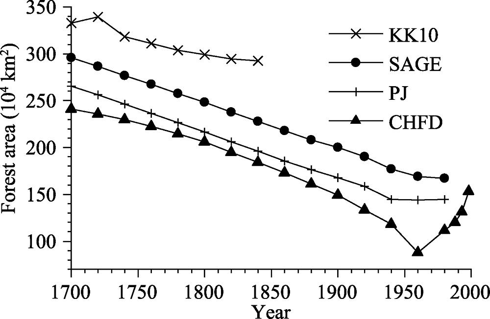
The trend of change in forested areas since the year 1700 represented by the datasets reflected a decrease, but estimates for forested areas varied widely between the global scenarios and regional results for China as illustrated in Figure 1.

Forest areas across China in CHFD between 1700 and 1960 underwent a rapid decrease, with a loss of 64% of the area from 1700 and a forested area dynamic degree of -2.45%. The sharpest increase in the forested area was observed during 1960-1998 by 83%, with a forested area dynamic degree of 21.87%. Two stages of changes in forested areas were detected in both SAGE and PJ; a period of linear decrease from 1700 to 1940, with losses of 40% and 46% compared with 1700, and a forested area dynamic degree of -1.68% and -1.90%, respectively, with a slightly decreased or approximately constant area from 1940 to 1990. KK10 showed a slow decrease from 1700 to 1850, with a total decrease of about 10% and a forested area dynamic degree of -0.67%. The results indicate that changes in forested areas varied significantly between the global scenarios and CHFD.

Large differences in the area occupied by forests in China in the global scenarios and CHFD were observed (Table 2). The area occupied by forests in CHFD was 241.27×10⁴ km² in 1700, and had decreased to 87.88×10⁴ km² by 1980, while forested area in SAGE decreased from 296.00×10⁴ km² to 167.00×10⁴ km² during this period. The area occupied by forests in China for SAGE was 20%-40% more than that for CHFD; the maximum difference was 65% in 1960. At the same time, the forested area in PJ decreased from 241.27×10⁴ km² to 143.98×10⁴ km², closer to that in CHFD than in SAGE. The relative biases in most time slices among them were lower than 20%—only in 1960 did the relative bias reached 49%. From 1700 to 1840, the forested area in KK10 was 292.50×10⁴ km²-339.63×10⁴ km², and 184.11×10⁴ km²-241.27×10⁴ km² in CHFD. The former was 32%-46% greater than the latter.

Overall, SAGE and KK10 overestimated the forested area from 1700 to 1990 across China, and changes in areas occupied by forests varied significantly between them. PJ was closer to CHFD in terms of total forested area.

To further reveal the uncertainty in the global scenarios, this study compared them with CHFD at the provincial scale. The comparison in Section 3.1 shows that the total forested area in PJ was the closest to that of CHFD among the global scenarios. Therefore, we carried out a provincial evaluation of only PJ.As shown in Figure 2, 13 provinces in PJ exhibited the same trend, as evident across China, featuring a phase of rapid linear decrease followed by a slight decrease. Forested area in 10 provinces decreased more than those in CHFD. For instance, the forested area dynamic degree of Shaanxi Province over this 300-year period in PJ was -1.55%, with a decrease of 43% in terms of area compared with that in 1700. The dynamic degree and decrease in forested area for the same province in CHFD were -0.45% and 13%, respectively. The decreases in forested area in Jing-Jin-Ji (Beijing-Tianjin-Hebei), Jilin, and Chuan-Yu (Sichuan-Chongqing) were smaller than in CHFD. In Jilin, for instance, CHFD had a forested area dynamic degree of -1.82% through the entire period, and the reduction of forested area as recorded by it was 51%, while the dynamic degree and reduction in forested area of this region according to PJ were -1.04% and 29%, respectively.

In the PJ scenario, eight provinces exhibited a slow decrease in forested area: Inner Mongolia, Heilongjiang, Fujian, Yunnan, Tibet, Gan-Ning (Gansu-Ningxia), Qinghai, and Xinjiang. The dynamic degrees of their forested areas were between -0.93% and -0.27%. This trend was significantly different from that of CHFD. In the past 300 years, for example, the forested area dynamic degree of Heilongjiang Province in CHFD has been -1.62%, and its forested area has decreased by 45%, whereas the dynamic degree and decline in forested area for this province in PJ were -0.68% and 19%, respectively. The comparative results suggest that 21 provinces recorded significant variations in forested area, accounting for 84% of all provinces considered.A total of 23 provinces reflected large differences in area between PJ and CHFD, accounting for 92% of all provinces. The forested areas of 14 provinces in PJ were considerably greater than their counterparts in CHFD. From 1700 to 1980, for instance, the forested area of Hu-Ning (Shanghai-Jiangsu) was between 0.09×10⁴-0.50×10⁴ km² in CHFD, and 1.70×10⁴-6.76×10⁴ km² in PJ, a difference as high as 170%-290%. In PJ, seven provinces had forested areas smaller than those in CHFD: Jilin, Chuan-Yu, Yunnan, Tibet, Gan-Ning, Qinghai, and Xinjiang. Throughout this period, for instance, the forested area of Qinghai Province was between 0.20×10⁴-4.98×10⁴ km² in CHFD, and 0.01×10⁴-0.03×10⁴ km² in PJ, a difference of 280%-520%. Only the forested areas of Liaoning and Hunan in PJ were closer to those in CHFD, with differences of -15%-22% and -6%-5%, respectively.The provincial evaluation indicates that 84% and 92% of the provinces had large differences in terms of trend and quantity, respectively, between PJ and CHFD. Therefore, there were significant discrepancies between them at the provincial scale.

3.3.1 Comparison of overall spatial pattern

Figure 3 illustrates the overall spatial pattern of forest cover in the PJ and CHFD datasets as well as the relative differences between them. As is shown, the spatial distribution of forests in PJ was in general agreement with that in CHFD, and both showed that eastern China was dominated by forest cover. However, the forest coverage of PJ in the traditional cultivated region of China was significantly greater than that of CHFD. The data in CHFD featured a smaller forest coverage in the North China Plain, the middle lower Yangtze River, and the Loess Plateau than that in PJ because these regions, as traditional cultivated regions of China, had been subjected to high-intensity and large-scale anthropogenic disturbance over long periods. This resulted in large-scale deforestation before the Qing Dynasty. By contrast, these regions in the PJ scenario had a large amount of forest for the entire study period.

In data for the last 300 years, large differences in the range and magnitude of deforestation between PJ and CHFD were found. In CHFD, the forested area decreased significantly in the southwest, northeast, and southeast of China, which accurately captured the spatial and temporal differences in deforestation. For instance, the Qing government had adopted a series of policies to attract immigrants into Sichuan to carry out land reclamation in the late 17th century, leading to a significant loss of local forest cover (He et al., 2015). In the mid-19th century, the Qing government abolished its “Prohibit reclamation in Northeast China” policy, and the immigrant population increased exponentially in northeastern China (including Heilongjiang, Jilin, and Liaoning) (Yang et al., 2019). As a result, northeastern China became the area with the highest deforestation after southwestern China. By contrast, due to the use of the linear back-scaling reconstruction method, the forested area in PJ decreased at a constant rate, and thus there were no significant spatiotemporal differences in the range and magnitude of deforestation.In addition, extensive relative biases are shown in Figure 3c. Positive differences were distributed mainly in the North China Plain, the middle lower Yangtze River, and Loess Plateau, and indicated the overestimation of forested areas in PJ for these regions. The positive differences increased over time and were detectable throughout eastern China by 1960. The negative differences in western Sichuan and southeast Tibet reflected the underestimation of forested areas in PJ for these regions. It is clear that the main reason for the extensive relative differences was that deforestation in PJ tended to be represented as uniform.3.3.2 Relative biases on grid cell scaleAs shown in Table 3, the percentages of grids with relative biases under 30% (intervals -30%-0% and 0%-30%) were between 10%-26%, and only 3%-9% of grids had relative biases lower than 10%. Grids with relative biases over 70% (intervals >70% and <-70%) accounted for 60%-80% of all grids, and those with relative biases higher than 90% accounted for 55%-75%. The number of grids with large differences increased over time. In 1720, grids with relative biases higher than 90% accounted for 55% of the total, and the proportion of grids with relative biases were lower than 10% accounted for 9%. By 1960, grids with relative biases over 90% exceeded 75%, and those with relative biases under 10% accounted for only 3%. Moreover, significant positive biases were detected between PJ and CHFD. The number of grids with positive biases accounted for more than 80% of all grids while negative biases grids were less than 20%.

Using the historical document-derived CHFD dataset, this study evaluated the reliability of data on forested areas in global historical land use scenarios at the gross, provincial, and grid scales. The main conclusions are as follows:

(1) A gross comparison showed that the reported forested areas varied widely between the global scenarios and CHFD, although the trend was identical in them. SAGE and KK10 overestimated the area occupied by forests in China over the past 300 years; the forested area according to SAGE since 1700 was 20%-40% more than that from CHFD, and that according to KK10 from 1700 to 1850 was 32%-46% more than that in CHFD. The forested area in PJ was closer in value to that in CHFD than SAGE and KK10, with a difference of less than 20%.

(2) The provincial and grid evaluations suggested large differences between the data in PJ and CHFD. Provinces with significant differences in terms of trend and quantity between PJ and CHFD accounted for 84% and 92% of all provinces, respectively. Grids with relative biases over 70% (intervals >70% and <-70%) and 90% (intervals >90% and <-90%) accounted for 60%-80% and 55%-75% of all grids, respectively.

(3) Compared with CHFD, data on forests in China in the global scenarios—SAGE, PJ, and KK10—were subject to great uncertainty. Differences in aims, data sources, and methods of reconstruction led to significant discrepancies among them. The authors chose remote sensing-derived modern LUCC data available at the global scale as the starting point of the reconstruction, and used the linear back-scaling method to obtain global historical agricultural areas. The reconstructed agricultural data were then overlaid on a map of potential vegetation to estimate the historical forested area. However, at the regional scale, data on forests in China were reconstructed through the analysis and verification of historical documents and survey statistics, and the results accurately reflected historical changes in forested areas in China.

Although our evaluations suggest that land cover data in these global scenarios were uncertain, the method for deducting areas of historical land use from potential vegetation to obtain changes in land cover remains feasible at the global or continental scale, and can be used as a reference for spatially explicit reconstruction in the future, given that the archaeological and paleoecological records capture only land cover at a given site. It is noteworthy that preparing reliable data on potential vegetation and historical land use is essential before using this approach. On the one hand, the potential vegetation data used in global scenarios are mostly based on simulations of the relationship between vegetation and the environment, and the results are uncertain. Using regional historical evidence (e.g., pollen, historical archives, or archaeological investigations) to modify the results of the simulations can contribute to better depictions of natural vegetation. On the other hand, significant progress has been made in reconstructing regional historical land use. The bottom-up approach, i.e., the reconstruction of historical land use from the regional to the global level, is an effective way to improve the reliability of land use data for global scenarios. For example, the Chinese historical cropland data reconstructed based on historical documents have been used in HYDE 3.2. As a result, taking full advantage of historical archives to reconstruct long-term LUCC data is essential for improving the reliability of global scenarios, and meets the needs of regional climatic and ecological simulations.

References

[1] et alRole of land cover changes for atmospheric CO2 increase and climate change during the last 150 years. Global Change Biology, 10, 1253-1266(2004).
[2] Forests in the long sweep of American history. Science, 204, 1168-1174(1979).
[3] . The clearing of the woodland in Europe//Thomas J W L. Man’s Role in Changing the Face of the Earth(1956).
[4] et alUsed planet: A global history. Proceedings of the National Academy of Sciences of the United States of America, 110, 7978-7985(2013).
[5] et alGlobal consequences of land use. Science, 309, 570-574(2005).
[6] et alForest change of China in recent 300 years. Journal of Geographical Sciences, 18, 59-72(2008).
[7] Main progress in historical land use and land cover change in China during the past 70 years. Journal of Chinese Historical Geography, 34, 5-16(2019).
[8] et alEvaluating the accuracy of Chinese pasture data in global historical land use datasets. Science China Earth Sciences, 61, 1685-1696(2018).
[9] et alComparisons of cropland area from multiple datasets over the past 300 years in the traditional cultivated region of China. Journal of Geographical Sciences, 23, 978-990(2013).
[10] A spatially explicit reconstruction of forest cover in China over 1700-2000. Global and Planetary Change, 131, 73-81(2015).
[11] et alSimulating global and local surface temperature changes due to Holocene anthropogenic land cover change. Geophysical Research Letters, 41, 623-631(2014).
[12] Sources and sinks of carbon from land-use change in China. Global Biogeochemical Cycles, 17, 1034(2003).
[13] Maximum impacts of future reforestation or deforestation on atmospheric CO2. Global Change Biology, 8, 1047-1052(2002).
[14] Deforestation, erosion, and forest management in ancient Greece and Rome. Journal of Forest History, 26, 60-75(1982).
[15] et alConstraining the deforestation history of Europe: Evaluation of historical land use scenarios with pollen-based land cover reconstructions. Land, 6, 91(2017).
[16] The prehistoric and preindustrial deforestation of Europe. Quaternary Science Reviews, 28, 3016-3034(2009).
[17] The effects of land use and climate change on the carbon cycle of Europe over the past 500 years. Global Change Biology, 18, 902-914(2012).
[18] et alHolocene carbon emissions as a result of anthropogenic land cover change. The Holocene, 21, 775-791(2011).
[19] Estimating global land use change over the past 300 years: The HYDE Database. Global Biogeochemical Cycles, 15, 417-433(2001).
[20] et alThe HYDE 3.1 spatially explicit database of human-induced global land-use change over the past 12,000 years. Global Ecology and Biogeography, 20, 73-86(2011).
[21] et alAccuracy assessment of global historical cropland datasets based on regional reconstructed historical data: A case study in Northeast China. Science China Earth Sciences, 53, 1689-1699(2010).
[22] et alReconstructing provincial cropland area in eastern China during the early Yuan Dynasty (AD1271-1294). Journal of Geographical Sciences, 28, 1994-2006(2018).
[23] Spatially explicit mapping of soil conservation service in monetary units due to land use/cover change for the Three Gorges Reservoir area, China. Remote Sensing, 11, 468(2019).
[24] et alEvaluation of global historical land use scenarios based on regional datasets on the Qinghai-Tibet Area. Science of the Total Environment, 657, 1615-1628(2019).
[25] et alA reconstruction of global agricultural areas and land cover for the last millennium. Global Biogeochemical Cycles, 22, GB3018(2008).
[26] . Global cropland and pasture data from 1700-2007(2012). http://www.geog.mcgill.ca/~nramankutty/Datasets/Datasets.html
[27] Estimating historical changes in global land cover: Croplands from 1700 to 1992. Global Biogeochemical Cycles, 13, 997-1027(1999).
[28] ISLSCP II historical croplands cover, 1700-1992. In: Hall F G, Collatz G J, Meeson B et al. ISLSCP Initiative II Collection. Tennessee: Oak Ridge National Laboratory Distributed Active Archive Center, 1-20(2010).
[29] et alThe global distribution of cultivable lands: Current patterns and sensitivity to possible climate change. Global Ecology and Biogeography, 11, 377-392(2002).
[30] Study on the methods of land use dynamic change research. Progress in Geography, 18, 81-87(1999).
[31] et alLand use, land-use change, and forestry//IPCC Special Report-Summary for Policymakers. IPCC(2000).
[32] et alCO2 emissions from forest loss. Nature Geoscience, 2, 737-738(2009).
[33] et alExploring Spatiotemporal Pattern of Grassland Cover in Western China from 1661 to 1996. International Journal of Environmental Research and Public Health, 16, 3160(2019).
[34] et alStudy of the effects of land use on hydrochemistry and soil microbial diversity. Water, 11, 466(2019).
[35] Reconstructed cropland in the mid-eleventh century in the traditional agricultural area of China: Implications of comparisons among datasets. Regional Environmental Change, 13, 969-977(2013).
[36] Discussion on the index method of regional land use change. Acta Geographica Sinica, 58, 643-650(2003).
Fan YANG, Fanneng HE, Meijiao LI, Shicheng LI. Evaluating the reliability of global historical land use scenarios for forest data in China[J]. Journal of Geographical Sciences, 2020, 30(7): 1083
Download Citation