Contributing to the coherent nature, quantum walks behave in a different way from their classical counterparts. Quantum walks have a wide range of applications when first noted by Aharonov et al.^[1]. Their fast diffusive behavior can be applied to quantum search algorithms^[2]. Interestingly, quantum walks are basics for many fields, such as simulating quantum circuits^[3], describing quantum lattice gas^[4], exploring topological phenomena^[5–7], and simulating the energy transport in photosynthesis^[8,9]. According to whether the quantum walks are continuous or not, quantum walks can be classified to continuous quantum walks and discrete-time quantum walks (DTQWs). Experimental investigations of quantum walks have been demonstrated in trapped atoms^[10,11], trapped ions^[12,13], nuclear magnetic resonance (NMR)^[14], and photic systems. Particularly, various elements can be used to control photons and implement quantum walks, such as bulk optics^[6,15], waveguide structures^[16–22], and time-multiplexed framework^[23–25].

There are many means of classifying quantum walks, such as continuous quantum walks and DTQWs, according to the continuity of time, and one-dimensional (1D) and two-dimensional (2D) quantum walks according to the dimensionality of the walker that can arrive. Besides, we can also distinguish quantum walks on the basis of degrees of freedom, such as polarization, spin angular momentum (SAM), orbital angular momentum (OAM), and the path. In this review, we mainly discussed the photonic experimental realization of DTQWs in bulk optics and the time-multiplexed framework. We firstly overview the standard DTQWs theoretically in Section 2. Then, in the light of the experimental system structure, we introduce the realizations of quantum walks with bulk optics in Section 3 and the time-multiplexed framework in Section 4. Finally, we concluded and compared the experimental realizations of quantum walks in different photonic systems in Section 5.

First, let us briefly review 1D DTQWs on a line. Suppose there is a particle, whose bases are denoted by |↑〉 and |↓〉. Then, a flipping operation is applied to the coin Hilbert space (in this Letter, we take the Hadamard operation as an example), followed by a shift operation, which shifts the particle’s position to the right if the coin state is |↑〉 and to the left if the coin state is |↓〉. These two operations can be written as U^=S^C^,(1)where S^=∑x|↑〉〈↑|⊗|x+1〉〈x|+|↓〉〈↓|⊗|x−1〉〈x| (x=…,−2,−1,0,1,2,…,x represents the position) and C^=H^⊗I^ (H is a Hadamard operator: 12(111−1)) denote the shift operation and the coin flipping operation, respectively.

By iterating the above operation for t steps, the state of the system evolves to |Ψt〉=U^t|Ψin〉.(2)

With an initial state |Ψin〉=|↓〉⊗|0〉, three steps of this process are expressed as the following example: $$\begin{gathered} |Ψin〉→U^12(|↑〉⊗|1〉−|↓〉⊗|−1〉) \\ →U^12[(|↑〉⊗|2〉−|↑〉|↓〉)⊗|0〉+|↓〉⊗|−2〉] \\ →U^122(|↑〉⊗|3〉+|↓〉⊗|1〉+|↑〉⊗|−1〉 \\ −2|↓〉⊗|−1〉−|↓〉⊗|−3〉). \end{gathered}$$(3)

The whole system of quantum walks can be separated into coin space and walker space, as shown above. This means that at least two degrees of freedom are needed to act as the coin and walker, respectively. There are many degrees of freedom, such as polarization, SAM, OAM, and path, that can be easily controlled to realize quantum walks. In this section, under the consideration of freedom, we organize the implementation of DTQWs with OAM firstly. Moreover, this does not mean that quantum walks can be realized only with OAM, as we review below; other degrees of freedom that encode the coin state are also necessary. Then, there are a great many of experiments that use the degrees of freedom of path and polarization to encode walker position and coin states; we also summarize these experiments in this section.

As early as 1992, Allen et al.^[26] pointed out that photons in Laguerre-Gaussian (LG) mode light beams carry OAM with discrete values lℏ, where l is the helicity light phase fronts. Beam carrying OAM has unique phase and intensity profiles, which make it have great potentials in astronomic observation^[27], micro-manipulations^[28,29], stimulated emission depletion (STED)^[30], super-resolution imaging^[31], and so on. Since the quantum properties of OAM were first demonstrated by Mair et al.^[32] in 2001, more and more attention has been paid to exploring OAM of single photon for encoding high-dimensional quantum information. A large amount of experiments have been reported^[33–37].

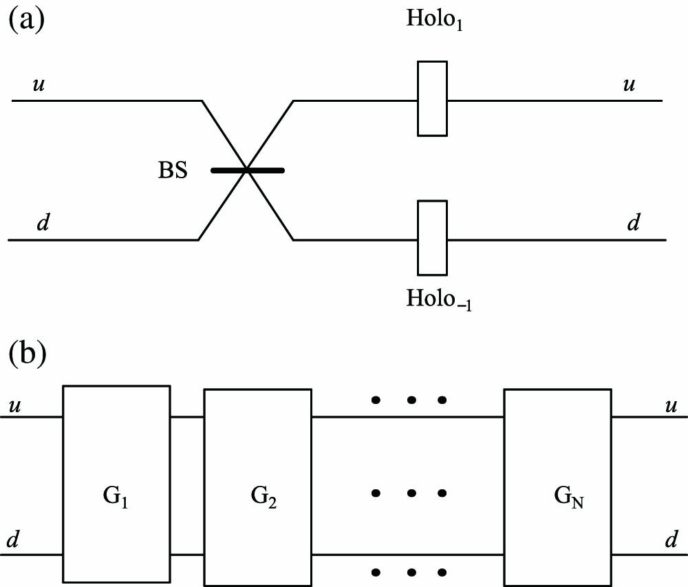
The above mentioned features provide a particularly suitable platform for implementing quantum walks. In 2006, Zou et al.^[38] first proposed an experimental scheme for implementing one-dimensional two-state quantum walks by using OAM of a single photon.

The experimental setup of one step of the one-dimensional two-state quantum walks is depicted by Fig. 1, where only a symmetric beam splitter (BS) and two computer generated holograms are used. The BS is used to implement the Hadamard operation of the coin states, through mixing the two optical modes (corresponding to the two paths of the pulse). The computer generated holograms are used to convert laser guided modes, which then change the OAM state from l to l±1. Then, one step is realized.

In 2007, Zhang et al.^[39] experimentally realized three steps of the quantum walks that depended on this scheme with some improvements. As we know, reflection by the mirror will change the helicity of light phase fronts, therefore changing the OAM of the photons from l to −l. A specially devised BS′ was used in this scheme. A BS′ (as shown in Fig. 2) consists of a normal symmetric BS and two mirrors. One of the mirrors is put in the upper input route and the other in the down output route of the BS. The BS′ performs a Hadamard operation on the spatial path (corresponding to the state of the particle) of the photon, and meanwhile the OAM remains unchanged, contrary to the situation when only a normal BS is used.

The two-level states are encoded by the two spatial paths of the photon pulse, and the position of the walker is represented by the OAM state. As aforementioned, the BS′ is used to flip the coin, and the computer generated hologram is used to demonstrate a shift operation by converting the OAM of the photon. The experimental setup is shown in Fig. 3. Three steps will be described in detail below.

Initial state: The state of the system is initialized and then incident to the setup, which is expressed as |↓〉⊗|0〉,(4)representing a photon of LG0 mode in the down route. Pinholes are inserted to filter for the first order of the diffraction of holograms.

Step 1: The first step of the quantum walks is implemented by BS1, Holo+1 in the upper path, and Holo−1 in the down path. BS1 performs a Hadamard operation on the coin state (path state), followed by Holo+1 and Holo−1 converting the OAM state of the photon from its initial state |0〉 to |+1〉 and |−1〉, respectively. Before entering BS2′, the state of the system evolves to 12(|↑〉⊗|1〉−|↓〉⊗|−1〉).(5)

Step 2: The upper and lower paths join in BS2′. No interference occurs here since the respective OAM states of the two paths differ. BS2′ performs a Hadamard operation on the path states. Two Holos here act similarly as in the first step. Thus, before entering BS3′, the state of the system evolves to 12[(|↑〉⊗|2〉−|↑〉|↓〉)⊗|0〉+|↓〉⊗|−2〉].(6)

Step 3: In the third step, because the same OAM state (|0〉) exists in both input states of BS3′, a Mach–Zehnder interference occurs here. Similar to former steps, Holo+1 and Holo−1 are placed in the upper and lower paths, respectively (Holos are not represented in the figure, which will be explained in the measurement step). The state of the system evolves to $$\begin{gathered} 122(|↑〉⊗|3〉+|↓〉⊗|1〉+|↑〉⊗|−1〉 \\ −2|↓〉⊗|−1〉−|↓〉⊗|−3〉). \end{gathered}$$(7)

Measurement: Single-mode fibers, holograms with proper ±l, and a power meter are used to collect photons and measure the energy of the output photons, from which the probability of photons in different positions can be calculated. It is known that only photons with OAM state |0〉 can propagate in a single-mode fiber (SMF). So, a Holo with proper l is placed before the coupler of the fiber to shift the OAM state to |0〉. For example, to measure a state |↑〉⊗|l〉, Holo−l, which transforms the state that will be changed to |↑〉⊗|0〉, is placed behind Holo+1 of BS3′. In the actual experiment, these two holograms can be combined to one for the sake of brevity.

Light beams have helical and polarization modes, corresponding to OAM and SAM for photons, respectively. When light transmits through an inhomogeneous and anisotropic medium, its OAM and SAM are not conserved separately. In particular, with a recently introduced photonic device called the “q-plate”^[40], the overall angular momentum can only be exchanged between OAM and SAM. The q-plate is essentially a retardation wave-plate made by a liquid-crystal birefringent medium with an inhomogeneous optical axis. Its special structure produces a topological charge q, so as to raise or lower the OAM of the photon crossing it according to its SAM. Using |↑,m〉 (|↓,m〉) denoting an initial state of a photon carrying mℏ OAM and ℏ (−ℏ) SAM, the action induced by a q-plate with q=0.5 can be represented as follows: $$\begin{gathered} |↑,m〉→q-plate|↓,m+1〉, \\ |↓,m〉→q-plate|↑,m−1〉. \end{gathered}$$(8)

As shown above, a q-plate performs only as a medium for the conversion between OAM and SAM, with the overall change of angular momentum nil. A q-plate with q=0.5 acts a “±1” on the OAM value m depending on the polarization. This spin-orbital system is a suitable carrier for implementing quantum walks (one conceptual scheme is illustrated in Fig. 4). In 2010, Zhang et al.^[42] proposed a scheme of 1D quantum walks by using photon SAM as the quantum coin and OAM space as the walk space. The experimental scheme is illustrated in Fig. 5.

The state of the photon can be expressed as |H,0〉=|R+L2,0〉,(9)where H represents horizontal polarization, and R and L represent the right circle polarization and left circle polarization, respectively. A set of wave-plates are used for the preparation of the initial state, followed by a gray box (shown in Fig. 5) that is used to flip the coin and then transform the position of the walker accordingly. The quarter-wave-plate (QWP) at 0° and half-wave-plate (HWP) at 22.5° of the box perform a Hadamard transmission (that is, a flip of the coin) to the coin state. Then, the q-plate in the box steps the photon to right or left by acting ±1 to the OAM value m. The HWP at 0° restores the spin. Thus, one step of quantum walks was realized.

Given an initial state |Ψin〉=|R,0〉, the first three steps evolve as $$\begin{gathered} |Ψin〉→U^12(|↑〉⊗|1〉−|↓〉⊗|−1〉) \\ →U^12[(|↑〉⊗|2〉−|↑〉|↓〉)⊗|0〉+|↓〉⊗|−2〉] \\ →U^122(|↑〉⊗|3〉+|↓〉⊗|1〉+|↑〉⊗|−1〉 \\ −2|↓〉⊗|−1〉−|↓〉⊗|−3〉), \end{gathered}$$(10)which is exactly the same as Eq. (3).

The probabilities of photons being in different positions can be measured with a similar method as in the aforementioned theme.

Compared with the scheme^[38,39] introduced previously, this scheme is more efficient and stable due to: first, a higher transmitted efficiency of 97% of q-plates compared to 37% of computer-generated holograms; second, there is no need for a phase-sensitive Mach–Zehnder interferometer. Based on these remarkable features, the steps of the quantum walks were estimated to reach 203 in the setup of Zhao et al.^[42].

In 2015, Cardano et al.^[41] experimentally implemented the scheme proposed in 2010^[42] by Zhang et al., both for a single photon and two simultaneous photons. The single-photon quantum walks were carried out with a set of apparatus similar to the classical one (using classical coherent light). It behaves equivalently to the classical one, resulting in the probability distributions being identical to the intensity distributions when using classical light. However, the setup introduced in this work is also suitable for investigation of multi-particle quantum interferences, which cannot be demonstrated classically. A two-photon quantum walk was designed to employ this feature. The experimental demonstration is briefly described below.

Photon pairs generated via type-II spontaneous parametric down conversion (SPDC) using a β-barium borate (BBO1) crystal are sent through a wave-plate set to initialize its state. Then, the two photons go through three identical subsequent quantum walk steps (similar to the part introduced in the previous scheme using classical light), followed by a 50:50 BS placed to randomly split them. The OAM state is then analyzed by diffraction on a spatial light modulator (SLM), followed by coupling into an SMF. Two interferential filters (IFs) are positioned before the SMFs to filter the photon band. The projection state corresponding to the OAM value is then fixed by the hologram pattern displayed on the SLM. Figure 6 shows the layout of the setup for the demonstration of a two-particle quantum walk.

A remarkable work reported more recently by Wang et al.^[7] in 2018 is introduced briefly below, as a typical example of the application of quantum walks demonstrated with OAM. In this work, the authors proposed and demonstrated the first, to the best of our knowledge, experiment for observation of topological phases in 2D quantum walks. In their experiment, the two degrees of freedom of the 2D quantum walks are encoded by spatial positions and OAM states of light. Based on this platform, the authors reported an observation of 2D topological bound states with vanishing Chern numbers. The experimental setup is illustrated in Fig. 7, consisting of three modules. Firstly, the initial state is prepared in the first module, as shown in Fig. 7(a). Then, many steps of 2D quantum walks are realized in the next module, as shown in Fig. 7(b). At the end of the setup, the results are detected by the last module, as shown in Fig. 7(c).

Quantum walks provide a powerful platform for simulating quantum phenomena. In particular, it is a suitable tool for observing and understanding topological phenomena, about which a lot of experimental observations have been reported. More examples on this can be found later in the Letter.

In this section, we will introduce several typical schemes using bulk optics with the freedom of polarization and path. As summarized in Ref. [43], these proposals with linear optical elements show that an inherent “quantum” system is not necessarily needed for implementing quantum walks, and the characteristic distribution of quantum walks can be effectively demonstrated using the interference of the classical field.

In 2002, Zhao et al.^[44] proposed one of the first schemes to implement 1D quantum walks with high feasibility using only linear optical elements. It also shows that a quantum walk tends to be classical when decohering the quantum states.

In this proposal^[44], the network for quantum walks is constructed with polarization BSs (PBSs) and HWPs. The quantum coin states are represented by the horizontal polarization state |H〉 and vertical polarization state |V〉 of photons. The PBS splits the input light into the two output ports denoted by “left” and “right” for |V〉 and |H〉, respectively. However, when a superposition state passes through the PBS from the “left” side, it goes wrong, since the |H〉 component is transmitted, and the |V〉 component is reflected. Thus, a PBS¯ consisting of a PBS and HWP (R90) is introduced to direct the |V〉 and |H〉 components correctly [see Fig. 8(b) for details]. Then, the movement of a photon can be defined depending on its polarization.

Figure 9 illustrates the optical setup constructed for implementing the quantum walks, where a network similar to Galton’s quincunx^[45] emerges. Each line in the figure is labeled by an integer j. Every single step results in the line changing from j to j+1. The optical elements along the jth line are labeled by k=−j,−j+2,…,j−2,j, representing position states |k〉.

The triangle in Fig. 9 represents elements and an input state, either |H〉 or |V〉, while the circle represents elements and two input states from the last line mixing here into a superposition state, followed by R45 (HWP at 22.5°) performing a Hadamard transformation: $$\begin{gathered} |H〉→12(|H〉+|V〉), \\ |V〉→12(|H〉−|V〉). \end{gathered}$$(11)

Then, PBSs and PBS¯s split the input state and pass them to the (j+1)th line. State |H〉 is transited to the “right” to the (k+1)th node of the (j+1)th line, while state |V〉 goes to the “left” to the (k−1)th node. By iterating the above procedure, quantum walks with arbitrary steps can be implemented by simply adding PBSs and PBS¯s.

A single-photon source is required in this scheme. Mature techniques such as SPDC^[46] and quantum dot^[47–50] can be chosen to demonstrate such a light source. By using a set of wave-plates^[51], an arbitrary initial state cosθ|H〉+eiψsinθ|V〉 can be prepared. The probability distribution feature of the quantum walks can be obtained by probabilistic measurement by putting detectors on the output path of the PBSs of the last line (represented by a square in Fig. 9).

In 2005, Do et al.^[52] experimentally realized a quantum quincunx by using linear optical elements. The arrangement depicted in Fig. 10 is similar to the original one proposed by Zhao et al.^[44], but does not require the specially defined optical element PBS¯. Another significant difference is a lower intensity He–Ne laser rather than a genuine single-photon source being used.

In 2010, Broome et al.^[15] experimentally demonstrated quantum walks with single photons. This experimental demonstration was also carried out based on the proposal of Zhao et al.^[44], and has one favorable feature that the number of optical elements required in this scheme scales linearly with the number of steps, contrasting to scaling exponentially in the scheme of Do et al.^[52], which is achieved by utilizing a birefringent calcite beam displacer (BD) instead of a PBS as the main element to construct the interferometers. They also explored the transition between quantum and classical walks by introducing decoherence^[53–55].

As in the original proposal of Zhao et al.^[44], the coin states in this scheme are encoded in the polarization states |H〉 and |V〉 of the photon, while the position states are defined by the spatial modes |i〉 (i=0,±1,±2,…) (see Fig. 11). As mentioned above, BD instead of PBS (or PBS¯) of previous proposals was employed to construct the optical network. The optical axis of the BD is cut so that vertically polarized light is directly transmitted, and horizontal light undergoes a lateral displacement into a neighboring mode. Then, the shift of the position (denoted by |i〉) to the left and right can be represented by lateral displacement and direct transmission through the BD, respectively, i.e., |H,i〉→BD|H,i−1〉,|V,i〉→BD|V,i−1〉.(12)

The probability distributions of one step of the quantum walks can be obtained by detecting the photons using an SMF and a single-photon detector at each output position of the step (see Fig. 11).

Another favorable feature of this scheme is the realizability of introducing decoherence by adjusting the relative angle between adjacent BDs, resulting in a temporal lag Δt and a transversal mode mismatch Δx between interfering wave-packets [Fig. 11(c)]. The authors pointed that full decoherence appears when setting a relative angle of 10.5° between the BDs. In this case, the probability distribution of a classical random walk is obtained, as shown in Figs. 12(b) and 12(c).

More recently, Bian et al.^[56] experimentally implemented a quantum walk on a circle with single photons. Clockwise-cycling and counterclockwise-cycling walks were realized in their experiments. The “real” position means the shift of the quantum walks was realized in the space of their spatial modes, compared to those in “abstract” spaces in other schemes^{[13,42,41,57–59]}. Quantum walks on cycles with four and three nodes were experimentally realized. Setup for four nodes cycles as an example is as shown in Fig. 13.

In 2018, Xue et al.^[60] proposed a scheme to demonstrate arbitrary 2D quantum walks also in a real position space via bulk optical elements. Figure 14 shows the setup for implementation of arbitrary coined 2D quantum walks. Here is a brief introduction of the first step, which is realized by four stages, as an example.

State preparation stage: Photons generated via type-I SPDC are prepared in a coin state in a four-dimensional (4D) Hilbert space by passing through a PBS, a BD, and three HWPs. In this procedure, four possible states of the coin for 2D quantum walks are represented by combining two polarizations of a photon and two possible spatial modes. By setting three HWPs at certain angles, arbitrary coin states for 2D quantum walks can be initialized.

Coin flipping stage: A four-sided coin flipping operator of the 2D quantum walks can be decomposed by the “cosine-sine” decomposition^[61]. In this way, a 4×4 matrix of the flipping operator can be easily implemented with a set of linear optical elements in the form of the coin flipping stage, as shown in Fig. 14, consisting of four BDs and some wave-plates.

Shift stage: The conditional shift operator can be realized by only one BD, as shown in the shift stage of Fig. 14, of which the axis is perpendicular to the preceding ones, thus allowing the photons passing through it to be separated longitudinally according to their polarizations^[62].

Expansion stage: In the expansion stage, the dimension of the Hilbert space of the coin will be expanded by BDs and HWPs at 45°, in order to prepare enough spare modes ahead of time for the next step. As is shown in Fig. 14, four BDs are used for the expansion stage.

Thus, we need (up to) four BDs for the flipping stage, one for the shift stage, and four for the expansion stage. This means that the request for the amount of elements for realizing 2D quantum walks increases linearly with the number of the steps.

In 2019, Su et al.^[63] experimentally demonstrated DTQWs with the walker initialized in superposition states and experimentally investigated the effects on the spread speed of the quantum walks when initializing the walker’s state in different superposition states. One of the innovations in that paper is the encoding method, in which the authors creatively encoded the polarization states of single photons as the walker’s positions, while encoding two spatial routes |U〉 and |D〉 of the single photons as the coin states. The conditional shift operator can be implemented by two HWPs at 0° and another two at Δθ/2 and −Δθ/2, respectively, as shown in Fig. 15(a), while the coin operator can be implemented by a BS, as shown in Fig. 15(b).

The setup of the scheme is shown in Fig. 16, and the steps of the quantum walks, with the walker initialized in superposition states, are described specifically as follows.

As mentioned above, the position states are encoded by the polarizations of the photon, which then can be initialized by the two HWPs inserted on the output paths of the first PBS. The coin state of the walker is encoded by the path of the photon, which can be initialized by the first PBS followed by two QWPs and one HWP inserted on the input paths of the PBS. By passing through BS 2, a shift operator of the coin is implemented. Then, the photon enters loop 2 counterclockwise, and HWP 2 implements the walking operator, i.e., the rotation of δθ (−δθ) is applied to the polarization space of the photon. The first step of the walk is implemented at this point. Then, the photon re-enters BS 2, and a second coin toss is performed. The photon has a probability to enter loop 1, similar to the situation in loop 2. In loop 1, a rotation of δθ (−δθ) in the polarization space is performed by HWP 1. The photon then passes through BS 2 again and enters loop 2 to realize the next step. In addition, the photon has a probability of passing through BS 1 and being detected by the device in the D1 (D2) part.

Besides the spatial mode for bulk optics, a novel freedom of arrival time of photons can also be used to realize DTQWs. The first experiment of a time-multiplexed detector was reported by Ref. [64]. In this section, we reviewed time-multiplexed framework DTQWs. The most prominent characteristic of this framework is the usage of the freedom of time-bin encoding. Although the structure of most of these experiments are fiber-loop, Xu et al.^[65] realize DTQWs in free space. Besides, in consideration of the number of loops in the experiment, 2D DTQWs are easier to be realized than bulk optics.

As illustrated in Fig. 17, the signal was input to a 50:50 coupler. Then, these pulses become delayed under the different lengths of fibers. By iterating this setup, the pulse input to this setup was firstly separated to several pulses. Although this setup was used to implement the detection with photon number resolution, this experiment can be improved to realize quantum walks. As illustrated in Fig. 18, the polarization of photons can be rotated by flipping operators, which is realized by an HWP at the initial position x. After passing through the first PBS, the vertically polarized photon is reflected to a longer path with position x−1, while the horizontally polarized photon is transmitted to a shorter one with position x+1. When they arrived at the second PBS, the horizontally polarized photon goes faster than vertically polarized one by Δt=Δl/c,(13)where Δl is the path difference for different polarization, and c is the velocity of light in the medium. This process is the implementation of the shift operator. Then, these photons will return to the beginning through a loop circuit and repeat this process.

The first, to the best of our knowledge, experimental realization of a time-multiplexed quantum walk was reported by Silberhorn et al.^[23]. There, the five step quantum walk was implemented with a fiber network loop. The experimental scheme is shown in Fig. 19. A picosecond pulsed laser was used to generate wave packets of photons under the repetition rate of 1 MHz. The neutral filters can decay the initial mean photon number to 〈n〉initial=8(2). Then, after photons passing through a 50% BS and being coupled into the fiber network, the mean photon number can reach the single-photon level. When coupled into the fiber, the vertically polarized photon takes 5 ns longer than the horizontally polarized photon. After being recombined at the second PBS, 50% of photons will be reflected out of the loop and detected, while the other 50% will take part in the next step walk. For this process, the single-photon level must be confirmed for the last step detection because the dead time of the avalanche photodetector (APD) may be too short to recognize that the photons come from the longer or shorter fibers.

In theory, the limitation of steps exists because the slowest photon of t−1 steps and the fastest photon of t steps must be distinguished. This limitation is related to the length of the longer fiber l1, shorter fiber l2, and the free space l. The rough relation under suitable repetition frequency is (N−1)(l1+l)<N(l2+l),(14)where N∈Z is the maximal steps for this setup. We can calculate the maximal steps as nine; however, only five steps were implemented in their experiment. The reason is that not only is the length of fiber but also the loss included in the detection limit walk steps. The efficiency of this setup is only ηsetup=0.18(1). Therefore, after five steps, the mean photon number decays to 〈n〉5steps≈7×10−4. For the sixth step, the average photon number will be too small to be distinguished from noise.

In the above example, a 1D quantum walk of five steps was realized. In 2011, further than this experiment, Silberhorn et al.^[24] realized a 28-step 1D quantum walk. This is obviously a very important development. As Fig. 20 shows, besides the reasonable length of fibers in Eq. 14, there are two factors that increased the steps. On one hand, a 12% BS was used to replace the 50% one. This replacement can allow more photons to return to the loop. On the other hand, they only guarantee the single-photon level at the last detected step, 〈n〉<0.003, rather than at the initial input state. This means that the classical laser can also be used to implement this experiment and end up with the same result. However, if we detect the classical laser at the last step, the dead time of the detector must be less than the time interval of the photons. Besides the 28 steps, the application of the electro-optic modulator (EOM), which is another development in the experiment, provides various possibilities to control the coin states. In this setup, on the basis of {|H〉=(1,0)T,|V〉=(0,1)T}, the matrix of the EOM is CEOM(x)=(eiϕH(x)00eiϕV(x)),(15)where ϕH(V)(x) represents a phase shift acting on |H(V)〉, and the arrival time can be regarded as the position x.

There exist various topological structures in multi-dimensional quantum walks. That means multi-dimensional quantum walks provide a platform to simulate lattice structure in condensed matter. Here, two examples are given to describe the 2D quantum walks by the fiber loop time-multiplexed framework. The first one is a 2D quantum walk simulation of two-particle dynamics reported by Silberhorn et al.^[25]. The walker is defined as |x1,x2,c1,c2〉, where x1 and x2 indicate its position in a 2D lattice, and c1 and c2 present its coin state. As Fig. 21 shows, incident photons follow, depending on their polarization, entering into four different paths, two for fibers and two for free space, to realize this 2D quantum walk. This optical fiber network realizes a 12-step 2D quantum walk and covers 169 positions in a 2D lattice. This work also provides a method to extend to more than two dimensions by adding loops in this network.

The other experimental realization of a delayed-choice 2D quantum walk was reported by Jeong et al.^[66]. This is the first, to the best of our knowledge, experiment that realizes a 2D quantum walk with a single-photon source in a time-multiplexed network. The experiment scheme is shown in Fig. 22, and although an entangled Bell state was prepared, only a single photon passes through the quantum walk network, namely Bob’s side, while the other photon is sent to Alice to implement delay choice. The difference of this 2D quantum walk from walking on the line above is that an extra freedom of the walk direction exists. They map the arrival time of photons to a 2D lattice of the walker. As shown in Fig. 22, two alternate directions, x and y, were introduced for alternate rotation operators, coin 1 and coin 2, which were realized by two HWPs. Firstly, a photon pair was generated via SPDC by a periodically poled KTiOPO₄ (PPKTP) crystal. It is quite different from previous decayed single photons; the photon sent to Bob was heralded in the measurement with the detection of the photon sent to Alice. However, this detection of coincidence count at two APDs has little difference from the experiment of quantum walks by bulk optics, which can be realized by continuous laser. In other words, only a pulse laser can be applied to produce photon pairs because the time interval of two photon pairs would be too short to exceed the dead time of APDs. But for the pulse laser, this time interval cannot be shorter than the period. In this experiment, the repetition rate of the laser is 1.25 MHz. The alternate directions x and y of the walker were implemented by a fiber loop and a free space loop, respectively. In the x step, the rotation is implemented by an HWP labeled coin 1, and the shift operator is implemented by a PBS, which can project the coin into two fibers L1 and L2 based on their polarization. After being recombined at the second PBS, the y-step walk starts at the rotation of coin 2, just the same as the x step, and the third PBS projects the coin into two paths of free space, L3 and L4. Finally, these photons reflected by the BS were detected, while the remaining photons returned to the loop and walked to the next step.

In this experiment, the coin operator is the Hadamard gate, H=(111−1)/2,(16)and the shift operators in the x and y directions are $$\begin{gathered} Sx=∑i,j∈Z|i−1,j〉W〈i,j|⊗|0〉C〈0| \\ +|i+1,j〉W〈i,j|⊗|1〉C〈1|, \end{gathered}$$(17)and $$\begin{gathered} Sy=∑i,j∈Z|i,j−1〉W〈i,j|⊗|0〉C〈0| \\ +|i,j+1〉W〈i,j|⊗|1〉C〈1|, \end{gathered}$$(18)where i(j) represents the lattice in the x(y) direction, and C and W indicate the coin and walker Hilbert space, respectively. Intuitively, if we want to implement a 2D quantum walk, it is necessary for a 4D coin space. After coin flipping, the walker will walk in four directions, left, right, up, and down, according to their coin state. In these programs, the walker can walk to any lattice on a 2D plane. Take the example of the Grove walk, the coin and shift operators are H=(−11111−11111−11111−1)/2,(19)and $$\begin{gathered} Sx=∑i,j∈Z|i−1,j−1〉W〈i,j|⊗|0〉C〈0| \\ +|i−1,j+1〉W〈i,j|⊗|1〉C〈1| \\ +|i+1,j−1〉W〈i,j|⊗|2〉C〈2| \\ +|i+1,j+1〉W〈i,j|⊗|3〉C〈3|. \end{gathered}$$(20)

The spatial distribution of the quantum walk described above is same, which has been proved in Refs. [67,68]. This means that split-step 2D walks can take the place of true multi-dimensional walks with multi-dimensional coins. For photons, it is too difficult to find an easily operated degree of freedom to encode multi-dimensional coins. Therefore, in this direct way, 2D quantum walks can be realized to explore quantum essence. The scheme provides a method to implement higher-dimensional quantum walks by a single qubit coin. Besides, the delay choice of this experiment shows that the polarization of the initial state is not decided, and the coincidence measurement with the ancilla chooses the valid initial state.

The topological protected edge state is fundamentally important in topological matter due to its robustness to various disturbances. The DTQWs provide a versatile quantum simulation platform to simulate the evolution of a time independent effective Hamiltonian. The motion of the walker can describe a particle on a discrete lattice, and the internal degree of freedom also can be simulated by the coin state. There are many explorations of topological phenomena of quantum walks theoretically and experimentally^[69,70]. Here, two examples of diverse experimental principles are given to describe the application of quantum walk in quantum simulation.

In the first example, Chen et al.^[71] observed the topologically protected edge state in a 2D quantum walk. A split-step quantum walk was introduced to describe the Floquet system when the periodic boundary exists for the walker. They use a spin-half-particle walking on a 2D lattice. The same as the realization of Ref. [25], alternative walk directions x and y are implemented for alternative coin rotations R(θ1) and R(θ2), and the unitary operator of a split-step quantum walk is U=TyR(θ2)TxR(θ1),(21)where R(θ)=e−iσyθ/2. x and y present the direction of the walker in a 2D lattice, and the shift operator in the x and y directions is $$\begin{gathered} Tx=∑x|x+1〉〈x|⊗|↑〉〈↑|+|x−1〉〈x|⊗|↓〉〈↓|, \\ Ty=∑y|y+1〉〈y|⊗|↑〉〈↑|+|y−1〉〈y|⊗|↓〉〈↓|. \end{gathered}$$(22)

Then, the effective Hamiltonian can be written as U=e−iH(θ1θ2)t/ℏ.(23)

The experimental implementation of this 2D quantum walk is shown in Fig. 23.

Although the main progress of this 2D quantum walk is similar to Ref. [25], the neoteric technique is that the usage of EOM can separate the space of x into two parts. For x<0, the angle of the EOM can be set as θ1,−, while, when x≥0, the angle of the EOM can be set as θ1,+. This spatial inhomogeneous quantum walk can investigate a nontrivial topological effect unique to a 2D driven system. They realized an inhomogeneous 2D quantum walk with 25 steps firstly. Although 28 steps have been realized by Schreiber et al. in Ref. [24], the walker covering a 2D 51×51 lattice is indeed in progress. There exist two factors that contribute to the progress in walking more steps. The first is the BS, reflecting 3% photons for detection, permitting more photons to return to the next step. When the parameters of the BS were reviewed, we can find that the smaller the reflected parameter, the more steps the walk can implement theoretically. However, when the reflected parameter is too small, the polarization influence on the BS will become more obvious, and the relative error of detection will be bigger. The second factor is the promotion of detection efficiency. The efficiency of superconducting nanowire single-photon detectors can be over 90%, while it is approximately 75% for the APD.

The results of probability distributions have been shown in Fig. 24(a). There is a localized probability distribution near the boundary at x=0 when the Hamiltonians H(θ1±θ2) belong to different topological phases. The P(B;n), which presents the probability of finding the walker in the boundary region, is shown in Fig. 24(b). It is obvious that if the edge state exists, P(B;n) tends to be a constant around 0.35; otherwise, P(B;n) declines with the evolution time. Figure 24(c) indicates that the spin of edge state direction is almost |↑〉 or |↓〉. The robustness of the edge state also be explored by applying a noisy EOM signal.

Another example of measuring the winding number in a large-scale chiral quantum walk was reported by Xu et al.^[65]. Although the detection of winding numbers had been explored^[71], this experiment provided a novel method for the framework of time multiplexing. On the contribution of their high time resolution technology in single-photon detection, the steps of the 1D quantum walk were pushed to 50 with nearly no photon losses before being detected at the last step. In this experiment, the time evolution operator is defined as U(θ1,θ2)=T−R(θ2)T+R(θ1),(24)where R(θ)=e−iσyθ is the coin operator, and T±:=∑x|x±1〉〈x|⊗|±〉〈±|+|x〉〈x|⊗|∓〉〈∓| is the shift operator.

The setup is shown in Fig. 25; it is quite different from the experiments above. No loop exists in this time multiplexing framework, and there is no extra photon loss in the walking process. There are two innovations that confirm this large-scale quantum walk. The first one is their quantum walks module, which is shown in Fig. 25(a). For each split step, after the rotation of the coin operator, which is implemented by an HWP, the horizontal photons will travel approximately 5 ps faster than the vertical ones for the birefringence in the calcite crystals; equivalently, the walker jumps to the right neighboring site when the coin state is horizontal. Then, the nest step was repeated to follow the same process. At the last step of this process, all arrival times of photons will be measured by their high time resolution technology, which is the other innovation. Because the time interval is 5 ps, it is too short to be distinguished by general time of digital converter. Therefore, detecting the coincidence count of the walker with a synchronizing signal or trigger is invalid. A creative method was designed to detect these time intervals. As Fig. 25(a) shows, the arrival time of signal photons is measured by scanning the pump laser and detecting the up conversion signals with photomultiplier tubes^[65]. The probability distribution of a Hadamard quantum walk is shown in Fig. 26. Then, on the basis of this large-scale quantum walk, the final state can be reconstituted by the application of quantum state tomography. Then, the winding number can be read out in different topological phases.

In this Letter we briefly introduced some typical experimental schemes of implementation of quantum walks in the photonic quantum system. Compared with other systems, the photonic quantum system has less requirement on environment (such as vacuum and low temperature), and photons can be easily manipulated through optical elements.

We first introduced the scheme of bulk optics, which are implemented mainly based on basic optical elements, i.e., PBS, q-plate, and various crystals, that can be commonly found in most optical laboratories. In schemes with bulk optics, the coin shift operators can be controlled more precisely, and even different shift operators depending on positions can be realized. However, it is difficult to implement a larger number of steps, as the scale of the optical structure increases rapidly with the increasing number of steps. Decoherence is the biggest challenge that needs to be overcome with the increase of the scale. While in the OAM scenario, a smaller optical structure is requested, since the positions are represented in the OAM space. Then, we introduced several schemes realized with the time-multiplexed framework. The advantage is that the number of the steps can be very large by implementing the quantum walks in the time domain. But at the same time, the flexibility of the implementation of the shift operator with different steps is low, which limits its applicable scenarios. These researches on experimental implementation of quantum walks provide multiple powerful experimental platforms for quantum algorithms, quantum computation, quantum simulation^[5,69,72], etc.