• Photonics Research
  • Vol. 10, Issue 9, 2147 (2022)
Mark A. Keppler1、2、*, Zachary A. Steelman3, Zachary N. Coker2, Miloš Nesládek4、5、6, Philip R. Hemmer7, Vladislav V. Yakovlev1、9, and Joel N. Bixler8
Author Affiliations
  • 1Department of Biomedical Engineering, Texas A&M University, College Station, Texas 77843, USA
  • 2SAIC, JBSA Fort Sam Houston, Texas 78234, USA
  • 3National Research Council Research Associateship Program, Washington, DC 20001, USA
  • 4IMOMEC Division, IMEC, B-3590 Diepenbeek, Belgium
  • 5Institute for Materials Research (IMO), Hasselt University, B-3590 Diepenbeek, Belgium
  • 6Czech Technical University in Prague, 27201 Kladno, Czech Republic
  • 7Department of Electrical and Computer Engineering, Texas A&M University, College Station, Texas 77843, USA
  • 8Bioeffects Division, Airman System Directorate, Air Force Research Laboratory, JBSA Fort Sam Houston, Texas 78234, USA
  • 9e-mail: yakovlev@tamu.edu
  • show less
    DOI: 10.1364/PRJ.455634 Cite this Article Set citation alerts
    Mark A. Keppler, Zachary A. Steelman, Zachary N. Coker, Miloš Nesládek, Philip R. Hemmer, Vladislav V. Yakovlev, Joel N. Bixler. Dynamic nitrogen vacancy magnetometry by single-shot optical streaking microscopy[J]. Photonics Research, 2022, 10(9): 2147 Copy Citation Text show less
    Intensity map (A) at the sample plane of a collection optic (B) is imaged to a narrow spatial mask (C) at the primary image plane. Individual colors indicate time steps. The mask constrains a single spatial dimension before the reduced intensity map is re-imaged to a detector by a 4f telescope (D). A galvo-scanner (E) at the telescope’s Fourier plane provides a constant velocity streaking operator, separating temporal information as a function of spatial position. The reduced and streaked scene is then imaged to the camera sensor (F) by the second 4f telescope lens where the information is encoded and digitized as a kymogram (G). Spatial masking minimizes the overlap between adjacent time steps on the detector after optical streaking. An example of an optically streaked sinusoidal magnetic field is displayed with corresponding y−t spatiotemporal coordinates. While results demonstrated below focus on microscopy, this general concept can be readily adapted to many imaging systems.
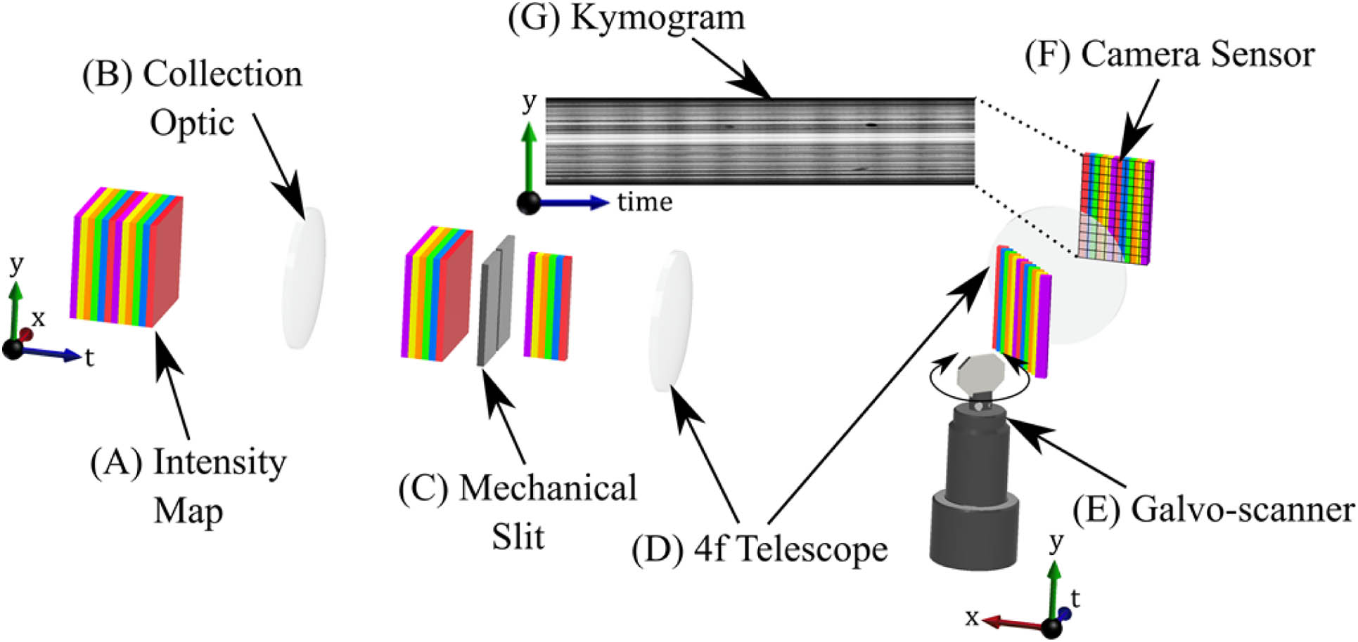
    Fig. 1. Intensity map (A) at the sample plane of a collection optic (B) is imaged to a narrow spatial mask (C) at the primary image plane. Individual colors indicate time steps. The mask constrains a single spatial dimension before the reduced intensity map is re-imaged to a detector by a 4f telescope (D). A galvo-scanner (E) at the telescope’s Fourier plane provides a constant velocity streaking operator, separating temporal information as a function of spatial position. The reduced and streaked scene is then imaged to the camera sensor (F) by the second 4f telescope lens where the information is encoded and digitized as a kymogram (G). Spatial masking minimizes the overlap between adjacent time steps on the detector after optical streaking. An example of an optically streaked sinusoidal magnetic field is displayed with corresponding yt spatiotemporal coordinates. While results demonstrated below focus on microscopy, this general concept can be readily adapted to many imaging systems.
    NV optical streaking magnetometer designed around a widefield fluorescence microscope is depicted. A 532 nm laser (green) was focused to the back focal plane of a long working distance objective (OBJ) by a plano–convex lens (L1). NV fluorescence (red) was separated from the source by a dichroic mirror (DM) and a long-pass filter LPF. The NV diamond sensor (NVD) was mounted on a printed circuit board with a co-planar microstrip RF antenna loop (RFA). An optical window at the center of the RF antenna allowed for illumination and fluorescence collection. A field coil (FC) was centered on the NV sensor such that spatially uniform magnetic fields could be generated. Spatially varying magnetic fields were generated with a permalloy electromagnetic needle (EM) wrapped with a coil fixed to a rotational mount. To reduce the amount of overlap between adjacent time steps, a mechanical slit (MS) was positioned at the primary image plane formed by the tube lens (L2). Optical streaking was achieved with a galvo-scanner (GS) positioned at the Fourier plane of a 4f telescope (L3 and L4) coupling the primary image plane to the detector (CMOS). Cylindrical beams and conic focal points are depicted to differentiate between infinity space and image planes, respectively. Components were not drawn to scale to assist with visibility of the optical path.
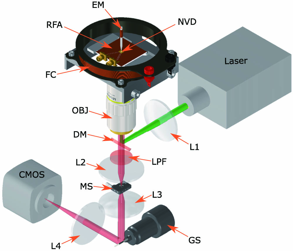
    Fig. 2. NV optical streaking magnetometer designed around a widefield fluorescence microscope is depicted. A 532 nm laser (green) was focused to the back focal plane of a long working distance objective (OBJ) by a plano–convex lens (L1). NV fluorescence (red) was separated from the source by a dichroic mirror (DM) and a long-pass filter LPF. The NV diamond sensor (NVD) was mounted on a printed circuit board with a co-planar microstrip RF antenna loop (RFA). An optical window at the center of the RF antenna allowed for illumination and fluorescence collection. A field coil (FC) was centered on the NV sensor such that spatially uniform magnetic fields could be generated. Spatially varying magnetic fields were generated with a permalloy electromagnetic needle (EM) wrapped with a coil fixed to a rotational mount. To reduce the amount of overlap between adjacent time steps, a mechanical slit (MS) was positioned at the primary image plane formed by the tube lens (L2). Optical streaking was achieved with a galvo-scanner (GS) positioned at the Fourier plane of a 4f telescope (L3 and L4) coupling the primary image plane to the detector (CMOS). Cylindrical beams and conic focal points are depicted to differentiate between infinity space and image planes, respectively. Components were not drawn to scale to assist with visibility of the optical path.
    (Left) Simplified block diagram demonstrating the streak control system. A PC data acquisition card provided the TTL signal to start the PGEN and serial communications with the RF generator. System timing was provided by a digital PGEN through TTL signals sent to trigger the camera and a function generator. Magnetic field and ramp voltages were output from the function generator to the magnetic field coil and galvo-scanner, respectively. Continuous RF was amplified before being coupled to the NV diamond by a coplanar microstrip antenna loop. (Right) The optical streak system timing diagram is shown for a single acquisition period T. Each waveform in the timing diagram is offset and referenced to a common voltage Vref for improved readability. (Red) “Galvo and Camera Timing” TTL pulse sequence output by the digital pulse/delay generator to initiate the galvo-mirror ramp and trigger the camera. The initial pulse starts the “Galvo-scanner Ramp” voltage (green) at the function generator. The width of the second pulse texp sets the acquisition time of the streak image. (Blue) Magnetic field control voltage output by the function generator triggered by the second TTL pulse. The magnetic field output is triggered by the rising edge of the pulse sent to trigger the camera.
    Fig. 3. (Left) Simplified block diagram demonstrating the streak control system. A PC data acquisition card provided the TTL signal to start the PGEN and serial communications with the RF generator. System timing was provided by a digital PGEN through TTL signals sent to trigger the camera and a function generator. Magnetic field and ramp voltages were output from the function generator to the magnetic field coil and galvo-scanner, respectively. Continuous RF was amplified before being coupled to the NV diamond by a coplanar microstrip antenna loop. (Right) The optical streak system timing diagram is shown for a single acquisition period T. Each waveform in the timing diagram is offset and referenced to a common voltage Vref for improved readability. (Red) “Galvo and Camera Timing” TTL pulse sequence output by the digital pulse/delay generator to initiate the galvo-mirror ramp and trigger the camera. The initial pulse starts the “Galvo-scanner Ramp” voltage (green) at the function generator. The width of the second pulse texp sets the acquisition time of the streak image. (Blue) Magnetic field control voltage output by the function generator triggered by the second TTL pulse. The magnetic field output is triggered by the rising edge of the pulse sent to trigger the camera.
    Optimization and magnetic sensitivity analysis to demonstrate proper NV function as a magnetometer during optical streaking. (A) ODMR plot of the average intensity across each streak as a function of RF from 2830 to 2910 MHz acquired with an ∼10 μm slit width (N=200 averages). Zeeman peak splitting of 17 MHz can be observed corresponding to the DC bias field from a neodymium magnet. (B) Profile plot of the average fluorescence contrast across a streak image calculated at 2874 MHz (N=200 averages), indicated by the dashed vertical red line in (C). (C) Optical streaking under a spatially uniform 40 Hz magnetic field (N=1) shows optimal RMS intensity roughly at the steepest tangents to the ODMR curve. The RMS amplitude of the intensity profiles at each RF was calculated using Eq. (1). (D) Average RMS intensity acquired from kymograms (N=100 averages) while decreasing the coil driving voltage shows linear field sensitivity down to around 10 μT. Error bars represent standard deviation from the mean.
    Fig. 4. Optimization and magnetic sensitivity analysis to demonstrate proper NV function as a magnetometer during optical streaking. (A) ODMR plot of the average intensity across each streak as a function of RF from 2830 to 2910 MHz acquired with an 10  μm slit width (N=200 averages). Zeeman peak splitting of 17 MHz can be observed corresponding to the DC bias field from a neodymium magnet. (B) Profile plot of the average fluorescence contrast across a streak image calculated at 2874 MHz (N=200 averages), indicated by the dashed vertical red line in (C). (C) Optical streaking under a spatially uniform 40 Hz magnetic field (N=1) shows optimal RMS intensity roughly at the steepest tangents to the ODMR curve. The RMS amplitude of the intensity profiles at each RF was calculated using Eq. (1). (D) Average RMS intensity acquired from kymograms (N=100 averages) while decreasing the coil driving voltage shows linear field sensitivity down to around 10 μT. Error bars represent standard deviation from the mean.
    Demonstration of magnetic field intensity plots obtained by optically streaking an electromagnetic needle moving laterally across the NV diamond sensor and validation of needle size. (A) A 50% transparent image of a 1951 USAF resolution test target was registered with an image of the needle such that the tip was adjacent to the horizontal bars of group 3 element 3 with a known width of 49.61 μm. (B) Magnetic field profile near the electromagnet imaged with the slit open and the needle stationary quantified by the change in fluorescence contrast from the background streak. A vertical dashed yellow line indicates the slice of the image captured by the narrow slit. The magnetic field intensity drops off sharply as the sharpened tip of the electromagnet recedes from the NV sensor that supports the ∼50 μm diameter measured in (A). A kymogram in (C) shows 200 ms of a 5 pixel/ms streak rate acquisition of the electromagnet moving at ∼1 μm/ms from top to bottom. The kymogram displays spatial information about the needle transit across the vertical axis and temporal information along the horizontal axis. Intensities represent relative changes in the fluorescence contrast as the needle is modulated with a sinusoidal field. Vertical striations in (C) are produced by a 40 Hz field modulation. (D) Bandpass filtered profile plot following the electromagnet centroid trajectory, represented by the yellow dashed lines in (C), demonstrating a measured frequency of 39.7±1.2 Hz taken as the reciprocal of the average time between wave peaks and troughs.
    Fig. 5. Demonstration of magnetic field intensity plots obtained by optically streaking an electromagnetic needle moving laterally across the NV diamond sensor and validation of needle size. (A) A 50% transparent image of a 1951 USAF resolution test target was registered with an image of the needle such that the tip was adjacent to the horizontal bars of group 3 element 3 with a known width of 49.61 μm. (B) Magnetic field profile near the electromagnet imaged with the slit open and the needle stationary quantified by the change in fluorescence contrast from the background streak. A vertical dashed yellow line indicates the slice of the image captured by the narrow slit. The magnetic field intensity drops off sharply as the sharpened tip of the electromagnet recedes from the NV sensor that supports the 50  μm diameter measured in (A). A kymogram in (C) shows 200 ms of a 5 pixel/ms streak rate acquisition of the electromagnet moving at 1  μm/ms from top to bottom. The kymogram displays spatial information about the needle transit across the vertical axis and temporal information along the horizontal axis. Intensities represent relative changes in the fluorescence contrast as the needle is modulated with a sinusoidal field. Vertical striations in (C) are produced by a 40 Hz field modulation. (D) Bandpass filtered profile plot following the electromagnet centroid trajectory, represented by the yellow dashed lines in (C), demonstrating a measured frequency of 39.7±1.2  Hz taken as the reciprocal of the average time between wave peaks and troughs.
    Mark A. Keppler, Zachary A. Steelman, Zachary N. Coker, Miloš Nesládek, Philip R. Hemmer, Vladislav V. Yakovlev, Joel N. Bixler. Dynamic nitrogen vacancy magnetometry by single-shot optical streaking microscopy[J]. Photonics Research, 2022, 10(9): 2147
    Download Citation