Abstract
We have developed a numerical framework that allows estimation of coherence in spatiotemporal and spatiospectral domains. Correlation properties of supercontinuum (SC) pulses generated in a bulk medium are investigated by means of second-order coherence theory of non-stationary fields. The analysis is based on simulations of individual space–time and space–frequency realizations of pulses emerging from a 5 mm thick sapphire plate, in the regimes of normal, zero, and anomalous group velocity dispersion. The temporal and spectral coherence properties are analyzed in the near field (as a function of spatial position at the exit plane of the nonlinear medium) and as a function of propagation direction (spatial frequency) in the far field. Unlike in fiber-generated SC, the bulk case features spectacularly high degrees of temporal and spectral coherence in both the spatial and spatial-frequency domains, with increasing degrees of coherence at higher pump energies. When operating near the SC generation threshold, the overall degrees of temporal and spectral coherence exhibit an axial dip in the spatial domain, whereas in the far field, the degree of coherence is highest around the optical axis.1. INTRODUCTION
Nonlinear propagation of a laser pulse in a transparent nonlinear material produces large-scale spectral broadening, termed supercontinuum (SC) generation [1,2]. SC presents a unique source of ultrabroadband radiation, which finds numerous applications in nonlinear optics and photonics. SC generation is often regarded as a white-light laser; to this end, its coherence properties are of major importance, especially considering the generation of diffraction-limited beams with excellent focusability and ultrabroadband pulses that are compressible to the transform limit, i.e., down to the few optical cycle duration.
SC pulse trains generated in microstructured fibers are representative examples of stochastic pulse trains, for which the temporal and spectral coherence properties are typically partial. The pioneering studies of spectral coherence of fiber-generated SC made use of the Dudley–Coen coherence function [3,4], which is readily measurable but of first order in the sense that it depends on a single frequency (wavelength) only. A complete description of the temporal and spectral coherence properties of pulsed optical fields (up to second order in the classical sense) requires knowledge of the two-time and two-frequency correlation functions [5], known as the mutual coherence function (MCF) and the cross-spectral density (CSD) function. These two-coordinate functions can be constructed by using appropriate ensemble averages over temporal and spectral realizations of individual pulses taken from a pulse train. When evaluated at a single instant of time, the MCF reduces to the mean temporal intensity of the pulses, whereas the CSD evaluated at a single frequency gives the mean power spectrum. By a suitable normalization, the MCF gives the complex degree of coherence of light between any two instants of time, whereas a normalized form of the CSD gives the corresponding degree of coherence of light between two arbitrary frequencies. Knowledge of the MCF and CSD at a single plane allows one to predict the spatiotemporal evolution of the light field and to forecast the outcome of various optical experiments.
In recent years, the two-time and two-frequency coherence properties of fiber-generated SC pulse trains have been studied rather extensively using simulated field realizations in various excitation conditions to construct the appropriate correlation functions, and the subject is now well understood [6–10]. No such detailed studies have been conducted for SC light generated in bulk media, which is the topic of the present work. In the few existing studies of temporal coherence properties of bulk-generated SC [11,12], coherence was characterized as a function of the time delay only. While such an approach is appropriate for stationary light, it is inadequate for a full statistical description of pulsed light.
Sign up for Photonics Research TOC. Get the latest issue of Photonics Research delivered right to you!Sign up now
Simulation of SC field realizations in fibers is relatively straightforward because of the guided-wave nature of the field [1,4]. Diffraction effects become prominent in bulk media, and, as a result, one should expect that the temporal and spectral coherence of the SC changes also as a function of spatial position at the exit plane of the medium. Addition of the diffraction process in SC generation increases the complexity of calculations considerably. Nevertheless, due to recent increase in computational power, numerical simulation of individual fields undergoing SC generation is possible. SC generation in bulk media appears to be a complex process that involves an intricate coupling between spatial and temporal effects: diffraction, chromatic dispersion, self-focusing, self-phase modulation, and multiphoton absorption or ionization. As a result, the laser beam transforms into a narrow light channel, termed light filament, while simultaneously the temporal pulse may undergo dramatic transformations: pulse splitting or compression, pulse-front steepening, and generation of optical shocks [13]. These transformations together produce broadband radiation with a non-trivial angular divergence that is accompanied by the generation of colored conical emission [2,13]. Statistical studies of bulk-generated SC have uncovered spectral, temporal, and spatial correlations between SC components, showing that these correlations exhibit complex evolutions as functions of the pump pulse energy [14–16]. In this paper, we numerically study the different coherence properties of bulk-generated SC by means of the mutual coherence and CSD functions.
The paper is organized as follows. Relevant measures of second-order coherence are introduced in Section 2, and extended to the far zone in Section 3. Section 4 describes the numerical model for SC generation in bulk, while the numerical results of SC generation in sapphire are presented in Section 5 in the ranges of normal, zero, and anomalous group velocity dispersion. Section 6 contains a systematic study of coherence properties of bulk-generated SC, and some remarks and possible further direction of the work are presented in Section 7.
2. MEASURES OF SECOND-ORDER COHERENCE
Let us consider a pulse propagating in the forward direction and restrict coherence analysis only in the positive half-space . We denote the electric field of a single realization as in the time domain, and as in the frequency domain. Here, is taken to denote a lateral position at the exit plane of the bulk medium, and the two electric fields are connected by the Fourier relationship Note that in the following, all spectral domain quantities (fields) will be denoted by a tilde. The angular spectrum of the field is defined as in the time domain, and as in the frequency domain. Here, is the spatial-frequency vector, and, due to Eq. (1), the quantities and are also connected to each other via a Fourier relationship.
Second-order coherence functions are defined as ensemble averages over individual pulse realizations. In the spatial domain, the coherence properties of light between two space–time points and at the exit plane are characterized by the MCF Correlations between two space–frequency points and at the exit plane are characterized by the CSD function In the spatial-frequency domain, one can similarly define the temporal angular correlation function (TACF) and the spectral angular correlation function (SACF) In Eqs. (4)–(7), the asterisk denotes complex conjugation, and the angle brackets denote averages of the form where is an individual realization taken from the statistical ensemble. In the spatial domain, we define the temporal intensity of light as and the power spectrum as , i.e., the intensity information of the field is given by the diagonal of the correlation function. Correspondingly, in the spatial-frequency domain, the temporal intensity is , and the power spectrum is . The intensities and spectral densities can be used to normalize the correlation functions, such that These degrees of coherence in various domains are generally complex-valued, but their absolute values are bounded between zero and unity. These limits represent incoherence and complete coherence, respectively, between two points in a four-dimensional space. Fourier-type relationships between the coherence functions defined in Eqs. (4)–(7) can be written straightforwardly using Eqs. (1)–(3).
In this work, we restrict our attention to temporal and spectral coherence properties of SC light at a single spatial point , or at a single spatial frequency . In other words, we do not consider the two-point spatial or angular coherence properties of the pulse train but concentrate on its spatial and spatial-frequency auto-correlation functions. We make direct use of the definitions in Eqs. (4)–(7) by inserting simulated pulse realizations into them, instead of using the relationships between the different correlation functions to determine one from another. It is nevertheless instructive to insert Eq. (2) into Eq. (6), and Eq. (3) into Eq. (7), which yields and If we write , this relation shows that the spectral coherence properties of the field at any single spatial frequency depend on the spectral and spatial coherence properties of the field at all spatial points across the exit plane of the bulk medium. Similarly, the temporal coherence properties of the pulse train at any single spatial frequency depend on the spatial and temporal coherence of the field at all points in the exit plane. Corresponding conclusions in the time domain can be drawn from Eq. (13).
The position-dependent overall degrees of temporal and spectral coherence, and , are defined, respectively, as [17–19] and Correspondingly, the single-spatial-frequency angular degrees of temporal and spectral coherence, and , are defined, respectively, as and It is straightforward to show that for any and for any .
Measuring the two-time and two-frequency correlation functions of SC light directly is a rather difficult task. In principle one could measure individual pulse realizations and construct the MCF and CSD function using the basic definitions in Eqs. (4) and (5), but such measurements are complicated because of the complex temporal and spectral structures of the pulses [20]. The use of time-resolved Michelson interferometry has also been proposed [21,22] but not yet fully demonstrated. In the case of fiber SC, most of the information on second-order coherence properties has indeed been retrieved by somewhat indirect techniques [10].
3. PROPAGATION INTO THE FAR ZONE
The term angular in TACF and SACF is perhaps somewhat deceptive, as these functions (evaluated at a single spatial frequency ) do not describe temporal and spectral correlations in a fixed physical propagation direction directly. To illustrate why this is the case, we employ the spherical polar angles and , so that the wave vector in the direction of unit vector is given by where , and is the speed of light in vacuum. From Eq. (20), it is clear that in addition to being dependent on physical propagation angles, the spatial frequencies also change as a function of . We can express the position vector in the far zone in a similar manner, so that and we consider propagation of light into the positive half-space , and more specifically, to the far zone where propagation distance is much larger than the Rayleigh range , with being the effective radius of the beam at the exit plane. The spectral electric field at a position in the far zone is given by (see, e.g., Eq. (3.2-88) in Ref. [23]) where is the frequency-domain angular spectrum defined in Eq. (3), evaluated at spatial frequencies .
The CSD function at a spatial point in the far zone, which is the true measure of far-zone spectral coherence properties of the field, is defined in analogy with Eq. (5) as On inserting from Eq. (22), we have where is the SACF given by Eq. (7), evaluated at two different frequencies and , towards the same propagation direction . The spectral density in the far zone is given by and the complex degree of spectral coherence at a point in the far zone has the form The effective degree of spectral coherence at point , , is defined in analogy with Eq. (16), and it appears to have no simple relation to the spatial-frequency-domain effective degree of spectral coherence .
The relationship between the MCF in the far zone and the TACF defined in Eq. (6) is even less transparent. The temporal field at position in the far zone is which is analogous to Eq. (1). On inserting from Eq. (22), we have where represents retarded time. The single-point MCF in the far zone, defined as then takes on the form To evaluate from the time-domain realizations , one should first construct the SACF, express it as a function of spatial frequencies , and then apply Eq. (30). The temporal intensity and the complex degree of temporal coherence at a point in the far zone can then be evaluated, as well as the effective degree of temporal coherence . Again, there seems to be no simple relationship between and .
For sufficiently narrowband fields, one may approximate in and also write in Eqs. (24) and (30). Then the relationship between the far-zone CSD function and MCF and the angular correlation functions are simplified, and Eq. (30) becomes The relations simplify also for broadband fields provided that they are (at least approximately) cross-spectrally pure [24] in the far zone, in the sense that However, in our case, SC-generated pulses do not satisfy this condition, as their far-zone diffraction patterns appear distinctly colored.
4. NUMERICAL SIMULATION METHOD
In order to numerically investigate second-order coherence measures, we had to produce a statistically reasonable number of individual spatiotemporal electric field distributions at the exit plane of the nonlinear crystal. We chose a 5 mm thick sapphire crystal as a nonlinear material for SC generation. Sapphire is a widely used nonlinear material, which serves for generation of highly stable and reproducible SC spectra in the visible and near-IR spectral ranges; see, e.g., Refs. [2] and [25].
The single-pulse nonlinear propagation in bulk material was numerically simulated by solving a unidirectional nonparaxial propagation equation for the pulse envelope , in the frequency domain assuming rotational symmetry [26]: Here, is the vacuum permittivity, denotes the dispersion relation of the medium, and is the refractive index calculated from the Sellmeier equation [27]. Additionally, , where is the group index.
The nonlinear polarization and current source terms were computed in the space–time domain, with where and are the linear and nonlinear refractive indices, respectively, is the cross section for inverse Bremsstrahlung, is the effective electron collision time, is the density of neutral molecules, and is the density of free electrons in the conduction band.
The intensity-dependent photoionization rate was calculated from Keldysh’s theory with electron–hole mass ratio and assuming the band gap of sapphire to be [27]. Finally, free-electron generation was simulated using a rate equation describing the evolution of the density of electrons in the conduction band: where the terms on the right-hand side stand for photoionization, avalanche ionization, and recombination, respectively, with as the free-electron recombination time [28].
The numerical simulations were performed with 30 μm full width at half-maximum (FWHM) diameter and 100 fs FWHM duration input pulses having central wavelengths of 800 nm, 1300 nm, and 2000 nm, at varying pump pulse energy levels. These wavelengths were chosen to investigate coherence in three different dispersion regimes around the central wavelength of normal, zero, and anomalous group velocity dispersion, respectively. The relevant parameters of sapphire for these particular wavelengths are presented in Table 1.
| λ (μm) | 800 | 1300 | 2000 |
| n0 | 1.76 | 1.75 | 1.73 |
| g (fs2/mm) | +58.1 | +1.8 | −121.8 |
| K | 7 | 11 | 16 |
| n2 (×10−16 cm2/W) | 3.11 | 2.89 | 2.7 |
| σB (×10−22 m2) | 9.2 | 19.6 | 32.4 |
Table 1. Relevant Linear and Nonlinear Parameters of Sapphire Crystal at the Wavelengths of Interesta
In the following numerical simulations, we start from a transform-limited pulse and add one photon per frequency noise as is commonly applied in numerical simulations of SC generation in fibers [1,30], and additionally introduce 0.5% normally distributed energy fluctuations to mimic intrinsic laser pulse energy fluctuations. The seed for the random number generator is the same for different pulse ensembles (datasets) so as to reduce the impact of different noise fluctuations on coherence measures. The main impact on coherence measures comes from the energy fluctuations, while the one photon per mode noise does not produce any noticeable impact. The numerical grid size and discretization are the same for all the pulses.
5. SIMULATION RESULTS
Temporal dynamics and spectral broadening around the threshold of SC generation in a bulk medium are very sensitive to energy fluctuations of the incident pulse [31]. This is illustrated in Fig. 1, which shows the evolutions (in logarithmic scale) of on-axis intensity profiles and spectra at the output plane of the sapphire sample versus the pump pulse energy.
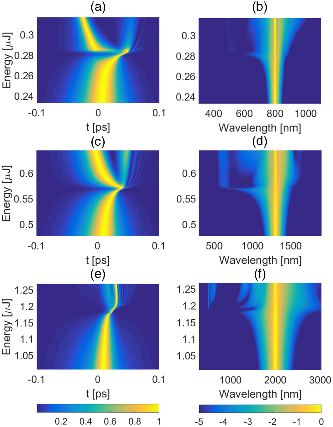
Figure 1.Evolution of the output pulse intensity and spectral density at the center of the beam as a function of pump pulse energy. (a), (c), (e) Temporal intensity and (b), (d), (f) spectral density. Here (a), (b) correspond to 800 nm, (c), (d) to 1300 nm, and (e), (f) to 2000 nm pump pulses.
It is noteworthy how narrow the energy intervals are where dramatic changes in the temporal and spectral domains occur. In Fig. 1, the left column shows the on-axis temporal pulse intensity profiles normalized to the maximum of each energy slice, whereas the right column represents the axial spectral distributions (in logarithmic scale) for the same pulses. Pulse splitting in the temporal domain is observed in the cases of normal and zero dispersion, while the pulse undergoes spatiotemporal compression in the case of anomalous dispersion. The pulse splitting or compression events are accompanied with abrupt spectral broadening, which marks the onset of SC generation. The threshold energies needed to generate SC in these conditions are 0.28 μJ, 0.56 μJ, and 1.175 μJ for pulses with central wavelengths of 800 nm, 1300 nm, and 2000 nm, respectively. In Fig. 1, it is clear that in the vicinity of the SC generation threshold, the temporal and spectral profiles of output pulses change a lot by a small change in input pulse energy.
The key difference from SC generation in fibers is the ability of the beam to self-focus during propagation in the material, which effectively generates many additional transverse modes especially in the nonlinear focus. The evolution of the beam radius upon propagation through the crystal is shown in Fig. 2 with pump energies of 0.282 μJ, 0.569 μJ, and 1.175 μJ for wavelengths of 800 nm, 1300 nm, and 2000 nm, respectively. These energies were chosen such that they are slightly above the threshold of SC generation and produce a nonlinear focus slightly before the output face of the crystal. Figure 2 also demonstrates that beams undergo a considerable shrinking before generating SC. Notice a somewhat different evolution of the beam radius [half width at half-maximum (HWHM)] in the case of anomalous dispersion (2000 nm), which is due to enhanced plasma absorption and defocusing, as the cross section of inverse Bremstanglung is larger for longer wavelengths.

Figure 2.Evolutions of beam radius over propagation distance for pulses with central wavelengths of 800 nm (blue), 1300 nm (green), and 2000 nm (red), having input energies of 0.282 μJ, 0.569 μJ, and 1.175 μJ, respectively.
In Fig. 3, we present the spatiotemporal intensity distributions and angle-wavelength spectral density distributions at the output plane of the crystal for the same input pulse conditions as in Fig. 2. The left column shows pulse intensity profiles as functions of radial distance and time, whereas the right column illustrates the resulting angle-resolved SC spectra. The non-trivial distributions of energy in spatiotemporal and angle-wavelength domains are evident and exhibit characteristic features of filamentation [2]. In what follows, these distributions are used to examine the second-order coherence properties by means of the correlation functions introduced in Section 2.
Figure 3.(a), (c), (e) Spatiotemporal intensity profiles of the pulses at the exit plane of a crystal and (b), (d), (f) corresponding spatial frequency-resolved spectra. Subplots (a), (b) correspond to 800 nm, (c), (d) to 1300 nm, and (e), (f) to 2000 nm pump wavelengths, having input energies of 0.282 μJ, 0.569 μJ, and 1.175 μJ, respectively.
6. APPLICATION OF SECOND-ORDER COHERENCE MEASURES ON NUMERICAL SIMULATION RESULTS
To examine the coherence properties of the wave packets, we have produced three datasets, each containing 100 realizations of nonlinear propagation, for input pulses with energies at the vicinity of the SC generation threshold for each pump wavelength (800 nm, 1300 nm, and 2000 nm). In the first dataset, most of the pulses did not produce SC (the average energy being slightly below the SC generation threshold). The second dataset contained almost equal fractions of pulses with energies that do or do not generate SC (the average energy coincides with SC generation threshold). In the third dataset, a vast majority of the pulses generated SC (the average energy being slightly above the SC generation threshold).
Figure 4 illustrates the correlation properties of a single dataset when SC was generated by 2000 nm pump pulses having energy slightly above the SC generation threshold. In Figs. 4(a) and 4(b), we demonstrate the absolute value of the single-point degree of temporal coherence defined in Eq. (9) at the exit plane of the bulk medium for two points in space: Fig. 4(a) represents the center () and Fig. 4(b) the periphery of the beam (). A cross-like modulation of temporal coherence evident in Fig. 4(a) represents lack of coherence at the steep front of the trailing part of the pulse; in this space–time region, pulse-to-pulse fluctuations are most prominent. In view of Fig. 4(b), the temporal coherence degree at the peripheral part of the beam is virtually perfect. The overall spatial degree of temporal coherence given by Eq. (15) is equal to 0.67 in the center part of the beam and 0.99 in the peripheral part. Therefore, loss of coherence occurs only within a small space–time volume close to the beam center.
Figure 4.Absolute values of normalized degrees of coherence. Spatial degrees of temporal coherence at (a) and (b) . Angular degrees of spectral coherence at (c) and (d) . Red curves show temporal pulse amplitude profiles in (a) and (b), and spectral amplitude profiles in (c) and (d).
In Figs. 4(c) and 4(d), we plot the absolute value of the single-spatial-frequency degree of spectral coherence defined in Eq. (12) at (on the optical axis) and off-axis position . For convenience, the results are plotted as functions of and . The on-axis spectral coherence is high around the pump wavelength and decreases towards both longer and shorter wavelengths. However, the overall angular degree of spectral coherence defined in Eq. (18) is 0.99 in the on-axis case, since the spectral amplitude of the pulses is significant only in the high-coherence region. In the off-axis case, the pulses are significantly wider in the spectral domain and asymmetric due to new spectral components generated via self-phase modulation, self-steepening, and plasma generation that eventually lead to SC. These are more prone to energy instability, which leads to a reduced overall degree of coherence .
To gain more insight into the spatial and angular degrees of temporal and spectral coherence, we now turn our attention to the behavior of the overall degrees of coherence defined in Eqs. (15)–(18). The use of these quantities in the spatial and spatial-frequency domains reduces four-dimensional correlation functions to one-dimensional line plots (because of rotational symmetry). In Fig. 5, the red curves show the overall degrees of coherence as functions of spatial position in Fig. 5(a) and spatial frequency in Fig. 5(b) for the output pulses generated at nine pumping conditions in the vicinity of the SC generation threshold. The blue curves show the normalized time-integrated pulse intensity distributions (fluence) in Fig. 5(a) and frequency-integrated spectral intensity distributions in Fig. 5(b).
Figure 5.Overall degrees of coherence at the exit plane, plotted as functions of spatial position (left, red) and spatial frequency (right, red) together with the corresponding normalized field intensity distribution (blue) integrated over time () and integrated over wavelengths (). The pump wavelength is 800 nm for the upper row, where we have considered pump energies just below the threshold at 0.277 μJ (solid), at threshold 0.280 μJ (dashed), and just above threshold 0.282 μJ (dotted). Similarly, for the 1300 nm pump wavelength in the middle row, the energies are 0.565 μJ (solid), 0.567 μJ (dashed), and 0.569 μJ (dotted), and at 2000 nm in the bottom row, they are 1.173 μJ (solid), 1.175 μJ (dashed), and 1.18 μJ (dotted). Note that the horizontal axes in the left column have different scales.
The dependence of the coherence measures on the radial spatial coordinate in Fig. 5(a) indicates that the lowest coherence occurs systematically at the center of the beam, where the fluence is highest. On the other hand, as seen in Fig. 5(b), the angular coherence is systematically highest in the axial region and decreases for off-axis components. These observations are in agreement with the trends already seen in Fig. 4 and can be explained as follows. The SC, having a broader spectrum at large spatial frequencies, is produced mainly at the center of a self-focused beam, where dramatic temporal transformations (splitting or compression) of the pulses take place. Therefore, this small spatiotemporal volume is most sensitive to small energy fluctuations between the incident pulses. This is particularly evident near the SC generation threshold, where the nonlinear propagation of the pulse ends just when SC is generated. In this situation, the generated spectral components are not spread far enough to affect coherence outside of the beam center.
In our analysis, we have deliberately chosen excitation conditions near the SC generation threshold for the output pulses to exhibit largest fluctuations in spatiotemporal and angle-wavelength domains, resulting in the drop of coherence at the beam center and at large spatial frequencies. We have also carried out additional numerical simulations for higher pump energies (well above the SC generation threshold but without filament refocusing or secondary pulse splitting) and computed the coherence measures for these data sets. These results are presented in the Appendix, and they demonstrate almost complete coherence regardless of the dispersion at the pump wavelength. This is in stark contrast to the SC generation in fibers, where an increase in pump power generally results in a dramatic loss of coherence [7]. To be precise, the increase in power may result in coherence enhancement in also fibers under particular operating conditions, as reported in an all-normal dispersion regime [32]. However, numerical simulations suggest that the coherence is lost again due to polarization noise [33].
It is necessary to emphasize that the coherence measures vary depending on whether we consider real propagation/diffraction angles or spatial frequencies, as was discussed in Section 3. The real angles are more physical, whereas the spatial frequencies are mathematically more convenient. In the discussion above we have chosen to consider spatial frequencies. To compare the two approaches, we show the spectral intensities at some hand-picked spatial frequencies and propagation angles (corresponding to the spatial frequency at pump wavelength ) for SC generation with 1300 nm pulses. The results are presented in Fig. 6, where the plots (top to bottom) compare spectral intensities at spatial frequencies of , , and (blue), and at corresponding physical propagation angles of 0.32 deg, 1.78 deg, and 3.6 deg (red) in ascending order. As expected, the spectral density difference between a particular real propagation angle and corresponding spatial frequency becomes prominent for higher propagation angles. Although the spectral density distributions exhibit substantial differences in this higher propagation angle region, the effects on coherence are minor, as shown in Fig. 7.
Figure 6.Comparison between the spectral density distributions taken at particular spatial frequencies (blue) and at corresponding real diffraction angles (red). Pump wavelength is 1300 nm. (a) , . (b) , . (c) , .
Figure 7.Comparison between the overall degree of coherence as a function of spatial frequency (, blue line), and as a function of real diffraction angle (, red crosses) calculated from the spatial frequency component at 1300 nm.
We have checked the angular correlation functions at some specific spatial frequencies and corresponding real diffraction angles. We present the comparison in Fig. 7. Here, the horizontal axis represents the real diffraction angle, and the vertical axis represents the overall degree of coherence. From the comparison, we can conclude that, though the spectral intensities may differ in fine detail, the overall degree of coherence stays almost the same in both representations even at large diffraction angles. This justifies our use of the spatial-frequency analysis approach.
7. CONCLUSION
In conclusion, we developed a numerical framework to estimate coherence in spatiotemporal and spatiospectral domains. We numerically studied the spatiotemporal and angle-wavelength coherence properties of bulk-generated SC by employing second-order correlation functions. The analysis is based on simulations of individual space–time and space–frequency realizations of pulses emerging from a 5 mm thick sapphire plate, using 100 fs pulses with carrier wavelengths of 800 nm, 1300 nm, and 2000 nm that fall into the ranges of normal, zero, and anomalous group velocity dispersion of sapphire, respectively, and using pump pulse energies around the respective SC generation thresholds. We have demonstrated that SC generation near the threshold is unstable, where small variations of input energy can drastically change the outcome. It was found that the lowest coherence occurs at the center of the beam and at the largest spatial frequencies. We have also discussed the angular frequency and diffraction angle differences in estimating coherence. In the future, we expect to verify these results experimentally, and also to provide more detailed studies on the effects of pulse length on the temporal and spectral coherence properties of SC. On the theoretical side, we also plan to analyze the spatial coherence of bulk-generated SC, the significance of space–frequency and space–time coupling, and topics such as the degree of cross-spectral purity of SC radiation.
APPENDIX A
Figure 8 presents the field intensity distributions integrated over time () and overall degrees of coherence as functions of spatial position for pump wavelengths of 800 nm, 1300 nm, and 2000 nm and for pump energies set well above their individual SC generation thresholds.
Figure 8.Overall degrees of temporal coherence calculated for pump energies well above the SC generation threshold: 0.31 μJ at 800 nm, 0.65 μJ at 1300 nm, and 1.25 μJ at 2000 nm. The notations are the same as in Fig. 5.
References
[1] J. M. Dudley, G. Genty, S. Coen. Supercontinuum generation in photonic crystal fibers. Rev. Mod. Phys., 78, 1135-1184(2006).
[2] A. Dubietis, G. Tamoauskas, R. Suminas, V. Jukna, A. Couairon. Ultrafast supercontinuum generation in bulk condensed media. Lith. J. Phys., 57, 113-157(2017).
[3] J. M. Dudley, S. Coen. Coherence properties of supercontinuum spectra generated in photonic crystal and tapered optical fibers. Opt. Lett., 27, 1180-1182(2002).
[4] J. M. Dudley, S. Coen. Numerical simulations and coherence properties of supercontinuum generation in photonic crystal and tapered optical fibers. IEEE J. Sel. Top. Quantum Electron., 8, 651-659(2002).
[5] I. A. Walmsley, C. Dorrer. Characterization of ultrashort electromagnetic pulses. Adv. Opt. Photon., 1, 308-437(2009).
[6] G. Genty, M. Surakka, J. Turunen, A. T. Friberg. Second-order coherence of supercontinuum light. Opt. Lett., 35, 3057-3059(2010).
[7] G. Genty, M. Surakka, J. Turunen, A. T. Friberg. Complete characterization of supercontinuum coherence. J. Opt. Soc. Am. B, 28, 2301-2309(2011).
[8] M. Erkintalo, M. Surakka, J. Turunen, A. T. Friberg, G. Genty. Coherent-mode representation of supercontinuum. Opt. Lett., 37, 169-171(2012).
[9] M. Korhonen, A. T. Friberg, J. Turunen, G. Genty. Elementary field representation of supercontinuum. J. Opt. Soc. Am. B, 30, 21-26(2013).
[10] M. Närhi, J. Turunen, A. T. Friberg, G. Genty. Experimental measurement of the second-order coherence of supercontinuum. Phys. Rev. Lett., 116, 243901(2016).
[11] I. S. Zeylikovich, R. R. Alfano. Coherence properties of the supercontinuum source. Appl. Phys. B, 77, 265-268(2003).
[12] G. Genty, A. T. Friberg, J. Turunen. Coherence of supercontinuum light. Progr. Opt., 61, 71-112(2016).
[13] A. Couairon, A. Mysyrowicz. Femtosecond filamentation in transparent media. Phys. Rep., 441, 47-190(2007).
[14] D. Majus, A. Dubietis. Statistical properties of ultrafast supercontinuum generated by femtosecond Gaussian and Bessel beams: a comparative study. J. Opt. Soc. Am. B, 30, 994-999(2013).
[15] M. Bradler, E. Riedle. Temporal and spectral correlations in bulk continua and improved use in transient spectroscopy. J. Opt. Soc. Am. B, 31, 1465-1475(2014).
[16] A. van de Walle, M. Hanna, F. Guichard, Y. Zaouter, A. Thai, N. Forget, P. Georges. Spectral and spatial full-bandwidth correlation analysis of bulk-generated supercontinuum in the mid-infrared. Opt. Lett., 40, 673-675(2015).
[17] P. Vahimaa, J. Tervo. Unified measures for optical fields: degree of polarization and effective degree of coherence. J. Opt. A, 6, S41-S44(2004).
[18] H. Lajunen, J. Tervo, P. Vahimaa. Overall coherence and coherent-mode expansion of spectrally partially coherent plane-wave pulses. J. Opt. Soc. Am. A, 21, 2117-2123(2004).
[19] K. Blomstedt, T. Setälä, A. T. Friberg. Effective degree of coherence: general theory and application to electromagnetic fields. J. Opt. A, 9, 907-919(2007).
[20] X. Gu, M. Kimmel, A. P. Shreenath, R. Trebino, J. M. Dudley, S. Coen, R. S. Windeler. Experimental studies of the coherence of microstructure-fiber supercontinuum. Opt. Express, 11, 2697-2703(2003).
[21] R. Dutta, J. Turunen, A. T. Friberg. Michelson’s interferometer and temporal coherence of pulse trains. Opt. Lett., 40, 166-169(2015).
[22] R. Dutta, J. Turunen, A. T. Friberg. Two-time coherence of pulse trains and the integrated degree of temporal coherence. J. Opt. Soc. Am. A, 32, 1631-1637(2015).
[23] L. Mandel, E. Wolf. Optical Coherence and Quantum Optics(1995).
[24] M. Koivurova, C. Ding, J. Turunen, A. T. Friberg. Cross-spectral purity of nonstationary light. Phys. Rev. A, 99, 043842(2019).
[25] M. Bradler, P. Baum, E. Riedle. Femtosecond continuum generation in bulk laser host material with sub-μJ pump pulses. Appl. Phys. B, 97, 561-574(2009).
[26] A. Couairon, E. Brambilla, T. Corti, D. Majus, O. de J. Ramírez-Góngora, M. Kolesik. Practitioner’s guide to laser pulse propagation models and simulation. Eur. Phys. J. Spec. Top., 199, 5-76(2011).
[27] M. J. Weber. Handbook of Optical Materials(2002).
[28] S. Guizard, P. Martin, P. Daguzan, G. Petite, P. Audebert, J. P. Geindre, A. Dos Santos, A. Antonnetti. Contrasted behaviour of an electron gas in MgO, Al2O3 and SiO2. Europhys. Lett., 29, 401(1995).
[29] A. Major, F. Yoshino, I. Nikolakakos, J. S. Aitchison, P. W. E. Smith. Dispersion of the nonlinear refractive index in sapphire. Opt. Lett., 29, 602-604(2004).
[30] R. G. Smith. Optical power handling capacity of low loss optical fibers as determined by stimulated Raman and Brillouin scattering. Appl. Opt., 11, 2489-2494(1972).
[31] D. Majus, V. Jukna, E. Pileckis, G. Valiulis, A. Dubietis. Rogue-wave-like statistics in ultrafast white-light continuum generation in sapphire. Opt. Express, 19, 16317-16323(2011).
[32] A. M. Heidt, J. S. Feehan, J. H. V. Price, T. Feurer. Limits of coherent supercontinuum generation in normal dispersion fibers. J. Opt. Soc. Am. B, 34, 764-775(2017).
[33] I. B. Gonzalo, R. D. Engelsholm, M. P. Sørensen, O. Bang. Polarization noise places severe constraints on coherence of all-normal dispersion femtosecond supercontinuum generation. Sci. Rep., 8, 6579(2018).


