
Wei-Xia Wu, Zhi-Gang Zheng, Yan-Li Song, Ying-Rong Han, Zhi-Cheng Sun, Chen-Pu Li. Directed transport of coupled Brownian motors in a two-dimensional traveling-wave potential[J]. Chinese Physics B, 2020, 29(9):
- Chinese Physics B
- Vol. 29, Issue 9, (2020)
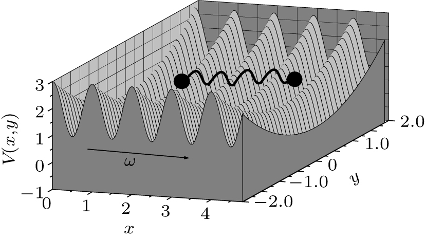
Fig. 1. Schematic diagram of coupled Brownian motors in the two-dimensional traveling-wave potential V (x ,y ).
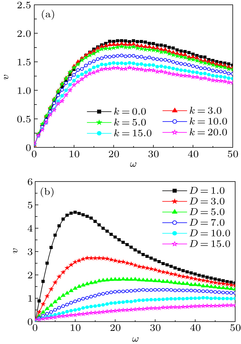
Fig. 2. The current υ versus the angular frequency ω for different values of (a) the coupling strength k at D = 5.0 and (b) the noise intensity D at k = 3.0, with other parameters being γ = 1.0, a = 5.0, V 0 = 3.0, λ = 3.0, and ε = 0.2.
Fig. 3. The current υ versus the wavelength λ for different values of the angular frequency ω , with other parameters being γ = 1.0, a = 5.0, V 0 = 3.0, k = 3.0, D = 5.0, and ε = 0.2.
Fig. 4. The current υ versus (a) the coupling strength k for different values of the angular frequency ω , and (b) the coupling strength k and the angular frequency ω with other parameters being γ = 1.0, a = 5.0, V 0 = 3.0, λ = 3.0, D = 5.0, and ε = 0.2.
Fig. 5. The current υ versus (a) the free length of the spring a for different values of the angular frequency ω , and (b) the free length of the spring a and the angular frequency ω , with other parameters being γ = 1.0, k = 3.0, V 0 = 3.0, γ = 3.0, D = 5.0, and ε = 0.2.
Fig. 6. The current υ versus (a) the noise intensity D for different values of the angular frequency ω , and (b) the noise intensity D and the angular frequency ω , with other parameters being γ = 1.0, k = 3.0, a = 5.0, V 0 = 3.0, λ = 3.0, and ε = 0.2.

Set citation alerts for the article
Please enter your email address
© Copyright 2018-2021 | Chinese Laser Press. All Rights Reserved 沪ICP备15018463号-20