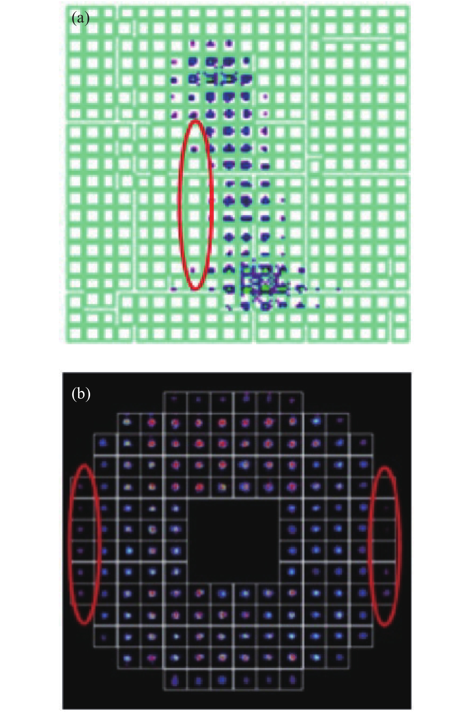
Fig. 1. Distribution of sub-aperture spot of different laser beams on the target of Shack-Hartmann-wavefront sensor. (a) slab laser beam cleanup; (b) DF chemical laser beam cleanup 不同激光束在夏克哈特曼波前传感器的子孔径光斑分布。(a) 板条激光器光束净化；(b) DF化学激光器光束净化

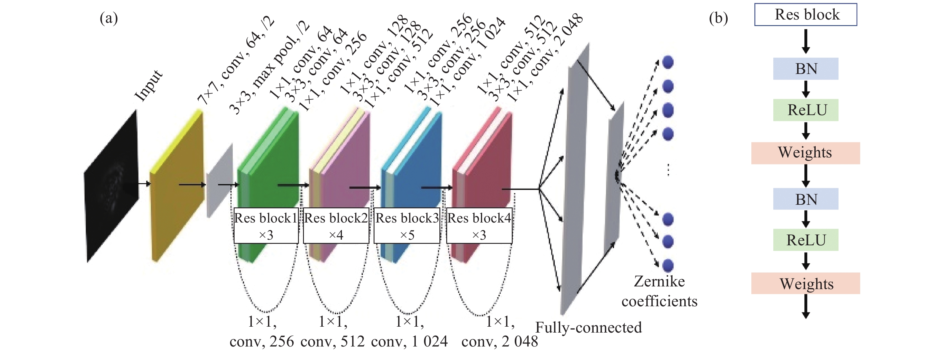
Fig. 2. ResNet-50 architecture to estimate Zernike coefficients. (a) Composition of the network; (b) Structure of residual block

Fig. 3. Schematic diagram of intensity distribution-based wavefront phase sensing with deep learning

Fig. 4. Wavefront aberration and correction result of a simulation data. (a) Input wavefront; (b) Reconstructed wavefront; (c) Residual wavefront after correction; (d) Intensity distribution of input; (e) Intensity distribution of reconstructed; (f) Comparison of actual Zernike coefficients and predict Zernike coefficients

Fig. 5. Turbulence phase screen and corresponding Hartmann detector sub-aperture spot distribution

Fig. 6. Structure of the optical system used in the experiment. Zernike coefficients and the corresponding far-field images are recorded by HSWFS and two CCDs

Fig. 7. Wavefront aberration and correction result of a experiment data. (a) Input wavefront; (b) Reconstructed wavefront; (c) Residual wavefront; (d) Intensity distribution of input; (e) Intensity distribution of reconstructed; (f) Comparison of actual Zernike coefficients and predict Zernike coefficients

Fig. 8. RMS of 1000 groups of verification data

Fig. 9. RMS of the Zernike coefficient (the piston and tilt terms excepted)

Table 1. Training result of the simulation data

Table 2. Training results with different noise

Table 3. Training results with different aberration

Table 4. Training results with different low-light areas

Table 5. Training result of the experimental data