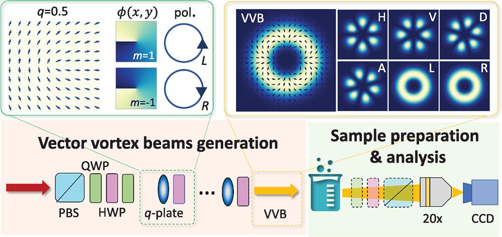
Fig. 1. Experimental scheme. A CW laser emits a Gaussian beam with m=0, at 808 nm. Then, the preparation stage for the initial polarization state is made with a PBS, QWP, and HWP. Five units, each composed of a q-plate (oval blue symbol) followed by an HWP (pink rectangle), generate structured light. Our q-plates display a charge q=0.5, which increases (decreases) the OAM number by 1. In the inset, we report the optical axis orientation of the plate and the phase acquired by the wavefront in the transverse plane ϕ(x,y) conditionally to the polarization states (L,R). After this preparation stage, we obtain VVBs in the form of Eq. (2), shown in the second inset of the figure (H, horizontal polarization; V, vertical polarization; D, diagonal polarization; A, antidiagonal polarization; L, left circular polarization; and R, right circular polarization). Depending on the analysis, we can use the whole vectorial field or the scalar fields produced by a suitable projection of the polarization on the basis b. The second stage consists of the sample, prepared with several concentrations of latex beads, and the detection platform. An objective collects the scattered light and focuses the image on the CCD camera. A polarization analyzer can be inserted between the sample and the objective.

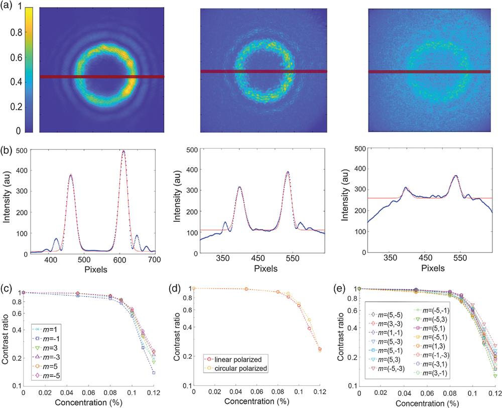
Fig. 2. Contrast analysis. (a) Recorded beam profiles associated with OAM 5 for three different concentrations C=0%, 0.10%, 0.12%. In each image, the red line indicates the selected slice for the fitting procedure. (b) Fit on the selected slices, for the same concentration of the above panel. Contrast ratio in a logarithmic scale for (c) circularly polarized OAM modes, (d) linearly and circularly polarized Gaussian modes, and (e) several VVBs modes as a function of the beads concentration, respectively.

Fig. 3. Depolarization analysis. (a) Pixel-by-pixel DR for the VVB mode with m1=5 and m2=−5, for three different concentrations C=0%, 0.10%, 0.12%. (b) Spatial profile of the same mode for comparison. (c) Pixel-by-pixel DR for a circularly polarized Gaussian mode, for three different concentrations C=0%, 0.10%, 0.12%. (d) Spatial profile of the same mode for comparison.

Fig. 4. Polarization pattern analysis. RGB map of the Stokes parameters for the VVB mode with m1=5 and m2=−5, for three different concentrations C=0%, 0.10%, 0.12%.

Table 1. Scattering properties of latex beads. The relevant parameters of our scattering samples are reported, namely the scattering length ls, transmission length ltr, scattering coefficient μs, the inverse of transmission length μs′, the scattering anisotropic coefficient g, and the quantity μsL, where L=1cm is the sample length. Those parameters are determined to provide a complete picture of the scattering conditions corresponding to the performed experimental tests. The values were retrieved for different concentrations C of latex beads. The calculations were obtained using the program available in Ref. 50.