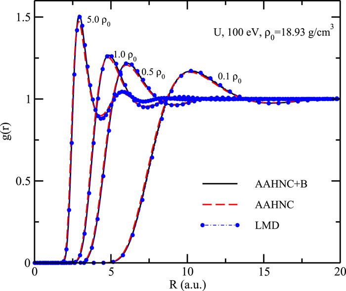
Fig. 1. Pair distribution functions as calculated with the AAHNC (red dashed lines), AAHNC+B (black solid lines), and LMD (blue dot-dashed lines with circles) methods as functions of the ion–ion distance for U at a temperature of 100 eV and densities of 1.893 g/cm³, 9.465 g/cm³, 18.93 g/cm³, and 94.65 g/cm³.

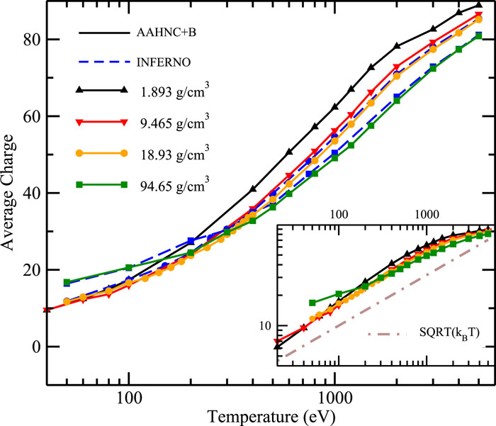
Fig. 2. Average charge of U as a function of temperature at solid density ρ₀ = 18.93 g/cm³ (circles), 0.1 × ρ₀ = 1.893 g/cm³ (triangles up), 0.5 × ρ₀ = 9.465 g/cm³ (triangles down), and 5 × ρ₀ = 94.65 g/cm³ (squares). Solid lines with different symbols represent the results for the different densities calculated using the AAHNC+Bridge model. The blue dashed lines with circles (18.93 g/cm³) and squares (94.65 g/cm³) are calculated using the INFERNO model.¹⁶ The inset shows a log–log plot along with the kBT behavior (brown dot-dashed line).

Fig. 3. Ionic coupling parameter Γ_ii for a hot dense U plasma as a function of temperature for densities in the range (0.1–5.0) × ρ₀.

Fig. 4. Pair distribution functions as derived from the AAHNC+Bridge method are shown as functions of the ion–ion distance for U at densities 1.893 g/cm³ (left), 18.93 g/cm³ (middle), and 94.65 g/cm³ (right) for different temperatures.

Fig. 5. Self-diffusion coefficient D (a) and shear viscosity η (b) of U as functions of temperature at different densities: 1.893 g/cm³ (dashed lines), 18.93 g/cm³ (solid lines), and 94.65 g/cm³ (dot-dashed lines). The CMD (black circles) and LMD (red squares) simulations are based on the effective pair potential from the AAHNC+Bridge calculations. For comparison, the results of OFMD (blue triangles up) simulations and the R–OCP model (green stars)¹⁶ are also shown.

Fig. 6. Stokes–Einstein relation F_SE as a function of temperature calculated from the diffusion coefficients and the shear viscosities at densities 1.896 g/cm³ (orange), 9.465 g/cm³ (black), 18.93 g/cm³ (red), and 94.65 g/cm³ (blue). The filled circles represent the results of LMD simulations and the open symbols those of CMD simulations. The gray dashed lines show the constant values of the Stokes–Einstein relation for stick (1/6π) and slip (1/4π) boundary conditions, respectively.