Hyperspectral Remote-Sensing Classification Combining Transformer and Multiscale Residual Mechanisms

Yuhan Chen; Bo Wang; Qingyun Yan; Bingjie Huang; Tong Jia; Bin Xue

doi:10.3788/LOP220921

Journals >Laser & Optoelectronics Progress >Volume 60 >Issue 12 >Page 1228002 > Article

Laser & Optoelectronics Progress
Vol. 60, Issue 12, 1228002 (2023)

Hyperspectral Remote-Sensing Classification Combining Transformer and Multiscale Residual Mechanisms

Yuhan Chen, Bo Wang^*, Qingyun Yan, Bingjie Huang, Tong Jia, and Bin Xue

Author Affiliations

School of Remote Sensing and Geomatics Engineering, Nanjing University of Information Science and Technology, Nanjing 210044, Jiangsu, China

show less

DOI: 10.3788/LOP220921 Cite this Article Set citation alerts

Yuhan Chen, Bo Wang, Qingyun Yan, Bingjie Huang, Tong Jia, Bin Xue. Hyperspectral Remote-Sensing Classification Combining Transformer and Multiscale Residual Mechanisms[J]. Laser & Optoelectronics Progress, 2023, 60(12): 1228002 Copy Citation Text

show less

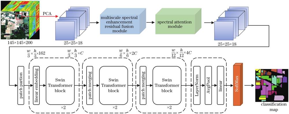
Fig. 1. Network structure of SMSaNet

Download full size

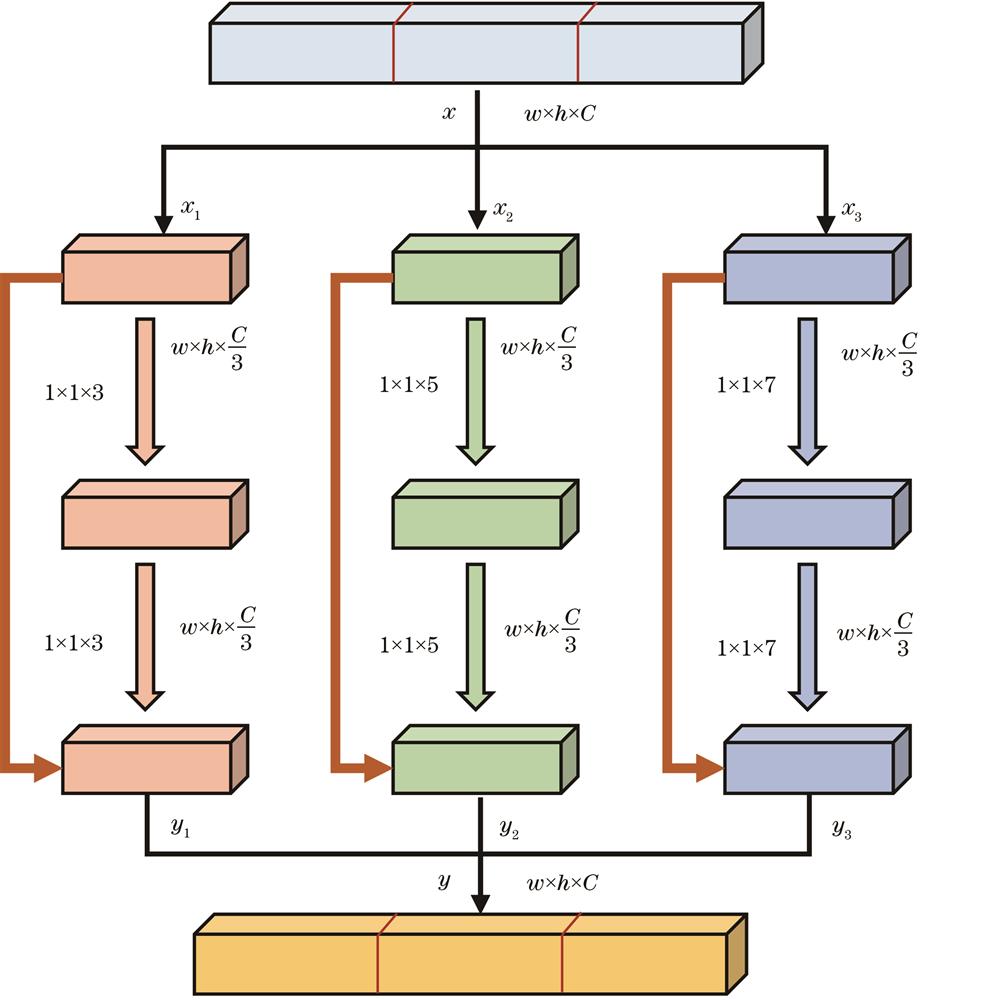
Fig. 2. Multiscale spectral enhancement residual fusion module

Download full size

Fig. 3. Spectral attention module

Download full size

Fig. 4. Swin Transformer feature extraction module

Download full size

Fig. 5. Swin Transformer block

Download full size

Fig. 6. MSA and W-MSA

Download full size

Fig. 7. W-MSA and SW-MSA

Download full size

Fig. 8. Classification result chart on India dataset

Download full size

Fig. 9. Classification result chart on PU dataset

Download full size

Fig. 10. Class activation mapping (CAM). (a) CAM of multiscale spectral enhanced residual fusion module; (b) CAM of spectral attention module

Download full size

Fig. 11. OA values corresponding to different ratios of training samples. (a) Inida dataset; (b) PU dataset

Download full size

Class No.	Land cover/use type	Training	Test
1	Alfalfa	23	23
2	Corn-notill	300	1128
3	Corn-min	300	530
4	Corn	118	119
5	Grass-pasture	241	242
6	Grass-trees	300	430
7	Grass-pasture-moved	14	14
8	Hay-windrowed	239	239
9	Oats	10	10
10	Soybean-notill	300	672
11	Soybean-mintill	300	2155
12	Soybean-clean	296	297
13	Wheat	102	103
14	Woods	300	965
15	Buildings-grass-trees-crives	193	193
16	Stone-steel-towers	46	47
Total		3082	7167

Table 1. Figure categories and sample counts of India dataset

Class No.	Land cover/use type	Training	Test
1	Asphalt	663	5968
2	Meadows	1864	16785
3	Gravel	209	1890
4	Trees	306	2758
5	Painted metal sheets	134	1211
6	Bare soil	502	4527
7	Bitumen	133	1197
8	Self-blocking bricks	368	3314
9	Shadows	94	853
Total		4273	38503

Table 2. Figure categories and sample counts of PU dataset

Dropout rate	0.1	0.2	0.3	0.4	0.5	0.6	0.7	0.8
OA /% （India）	99.47	95.60	99.51	97.41	98.23	99.01	98.44	96.91
OA /% （PU）	99.56	99.04	99.31	99.19	99.07	99.02	98.99	98.45

Table 3. Experimental results of different dropout rates on India and PU datasets

Spatial dimension	9×9	11×11	13×13	15×15	17×17	19×19	21×21
OA /%	97.92	98.51	98.93	99.02	99.22	99.21	99.33
AA /%	98.10	98.68	98.95	99.05	99.11	99.16	99.36
Kappa /%	98.21	98.51	98.73	99.17	99.25	99.31	99.34
Spatial dimension	23×23	25×25	27×27	29×29	31×31	33×33	35×35
OA /%	99.47	99.51	99.39	99.35	99.31	99.26	99.21
AA /%	99.52	99.66	99.45	99.26	99.18	99.15	99.10
Kappa /%	99.42	99.44	99.32	99.21	99.05	98.72	98.69

Table 4. Experimental results of different spatial sizes on India dataset

No.	Baseline	1D-CNN	3D-CNN	3D+2D-CNN	Swin-T	SMSaNet
1	96.77	100.00	100.00	100.00	100.00	100.00
2	77.91	78.15	98.60	98.70	96.44	98.95
3	70.16	74.39	99.32	98.97	98.80	99.48
4	66.83	68.45	100.00	100.00	98.22	99.09
5	93.43	91.57	100.00	100.00	99.41	99.85
6	95.38	95.95	99.41	99.61	99.22	99.80
7	95.24	86.36	95.24	90.91	100.00	100.00
8	99.11	98.82	99.41	100.00	100.00	99.85
9	68.75	70.59	100.00	100.00	100.00	100.00
10	79.55	77.82	99.27	99.27	97.84	99.85
11	90.81	88.87	99.53	99.47	99.76	99.33
12	74.07	65.96	99.52	98.54	97.42	99.76
13	99.28	97.92	100.00	100.00	100.00	100.00
14	97.22	97.92	97.77	99.77	99.77	99.89
15	76.55	72.99	96.09	98.54	95.07	98.90
16	93.65	91.18	98.46	100.00	100.00	99.22
OA /%	85.21	84.21	99.01	99.31	98.63	99.51
AA /%	88.99	89.13	98.45	99.44	98.74	99.66
Kappa /%	83.29	82.17	98.87	99.22	98.44	99.44

Table 5. Classification results on India dataset

No.	Baseline	1D-CNN	3D-CNN	3D+2D-CNN	Swin-T	SMSaNet
1	93.00	92.97	98.90	99.17	99.28	99.20
2	96.18	96.52	99.77	99.84	99.77	99.80
3	77.03	81.45	97.78	98.99	99.07	97.44
4	94.63	94.88	99.70	98.27	99.44	99.56
5	99.92	100.00	100.00	99.67	99.92	100.00
6	90.91	92.99	99.98	100.00	99.96	100.00
7	82.69	86.91	99.09	99.50	99.50	99.58
8	82.69	82.73	98.05	99.60	97.30	99.08
9	99.65	98.95	96.51	98.91	97.41	98.81
OA /%	92.66	93.40	99.32	99.54	99.38	99.56
AA /%	90.15	90.81	98.39	98.95	98.72	99.18
Kappa /%	90.26	91.23	99.10	99.39	99.18	99.41

Table 6. Classification results on PU dataset

Method and module				India			PU
Method	Shift	M	S	OA /%	AA /%	Kappa /%	OA /%	AA /%	Kappa /%
w/o shift		√	√	99.30	98.93	98.88	99.37	98.77	98.56
SMSaNet	√	√	√	99.51	99.66	99.44	99.56	99.18	99.41
w/o M	√		√	98.86	98.63	98.71	99.11	99.05	98.82
w/o S	√	√		99.21	99.16	99.13	99.28	99.09	98.87
w/o M and S	√			98.56	98.17	98.06	98.89	98.65	98.48

Table 7. Ablation experiments

Method	Image size	Param /M	FLOPs
Baseline	1×1	4.230	4.23 MFLOPs
1D-CNN	1×1	0.036	0.11 MFLOPs
3D-CNN	25×25	0.772	93.82 MFLOPs
3D+2D-CNN	25×25	5.009	152.68 MFLOPs
Swin-T	25×25	27.495	89.78 MFLOPs
SMSaNet	25×25	5.056	46.65 MFLOPs

Table 8. Params and FLOPs for different models

Download Citation

Set citation alerts for the article

Tools

Set citation alerts for the article

Save the article for my favorites

Paper Information