
Jianqiang Zhu, Jian Zhu, Xuechun Li, Baoqiang Zhu, Weixin Ma, Xingqiang Lu, Wei Fan, Zhigang Liu, Shenlei Zhou, Guang Xu, Guowen Zhang, Xinglong Xie, Lin Yang, Jiangfeng Wang, Xiaoping Ouyang, Li Wang, Dawei Li, Pengqian Yang, Quantang Fan, Mingying Sun, Chong Liu, Dean Liu, Yanli Zhang, Hua Tao, Meizhi Sun, Ping Zhu, Bingyan Wang, Zhaoyang Jiao, Lei Ren, Daizhong Liu, Xiang Jiao, Hongbiao Huang, Zunqi Lin, "Status and development of high-power laser facilities at the NLHPLP," High Power Laser Sci. Eng. 6, 04000e55 (2018)
- High Power Laser Science and Engineering
- Vol. 6, Issue 4, 04000e55 (2018)
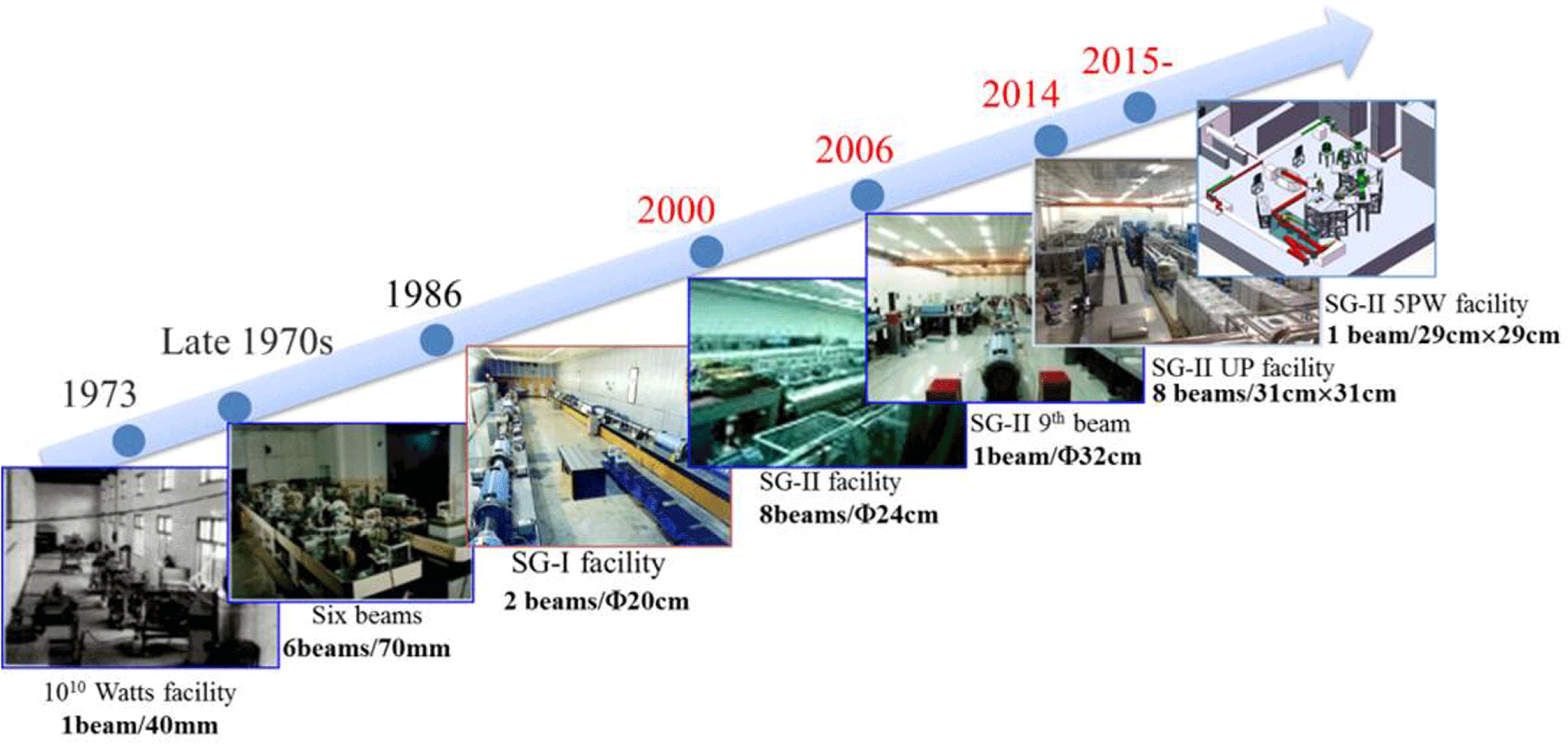
Fig. 1. Photographs of a series of laser facilities built at the NLHPLP.
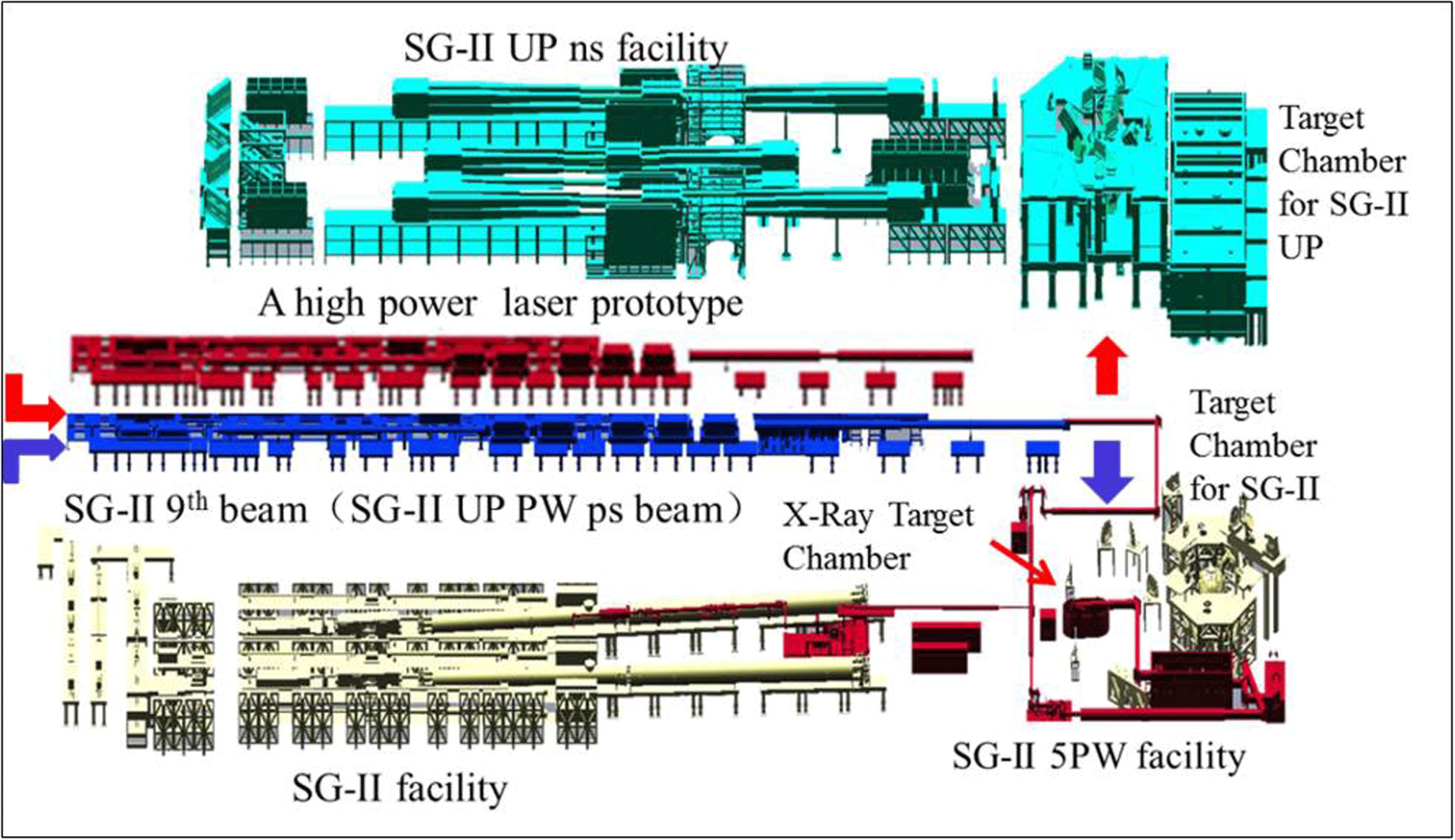
Fig. 2. Schematic view of the layout of the multifunctional platform.
Fig. 3. Operational shots of SG-II facility for physical experiments.
Fig. 4. Operational shots of SG-II UP facility for physical experiments.
Fig. 5. Photographs of the SG-II UP facility: (a) laser hall and (b) target chamber.
Fig. 6. Schematic of the optical layout of one beamline.
Fig. 7. Near-field fluence distributions of the $1\unicode[STIX]{x1D714}$ output (shot No. 20150721002): (a) near-field images and (b) fluence probability distribution.
Fig. 8. Far-field fluence distributions of the $1\unicode[STIX]{x1D714}$ output (shot No. 20150721002): (a) enclosed focal spot energy fraction and (b) far-field image.
Fig. 9. Experimental output capability for $1\unicode[STIX]{x1D714}$ with different pulse widths of the laser prototype.
Fig. 10. Experimental output capability of $3\unicode[STIX]{x1D714}$ with different pulse widths.
Fig. 11. Near and far fields of the $3\unicode[STIX]{x1D714}$ output measured by PDS: (a) near-field image, (b) far-field image, and (c) enclosed $3\unicode[STIX]{x1D714}$ focal spot energy fraction.
Fig. 12. $3\unicode[STIX]{x1D714}$ output energy per beam for four consecutive shots.
Fig. 13. $3\unicode[STIX]{x1D714}$ output power imbalance for eight beams (shot 4).
Fig. 14. Pulse shape in the (a) front end and (b) end of the main amplifier.
Fig. 15. Interface of Laser Designer and the comparison of the experimental and simulation results.
Fig. 16. (a) Regenerative amplifier, (b) output near-field profile, (c) energy stability of the regenerative amplifier for 8 h, and (d) square-pulse distortion of the regenerative amplifier.
Fig. 17. (a) Physical photograph of the optically addressed liquid crystal spatial light modulator and (b) demonstration of near-field spatial intensity control.
Fig. 18. Main amplifier of the SG-II UP ns laser facility.
Fig. 19. (a) CSF alignment package and (b) resultant image.
Fig. 20. TSF alignment package (top) and result images (bottom): (a) crystals, (b) TSF pass-1 pinhole, and (c) TSF pass-2 pinhole.
Fig. 21. Basic scheme for single-shot beam diagnostics in high-power laser systems with the CMI method.
Fig. 22. Comparison of the near-field intensity and phase: (a) near-field intensity reconstructed by the CMI method, (b) near-field intensity measured by direct imaging, (c) near-field phase reconstructed by the CMI method, and (d) near-field phase measured by a Shack–Hartmann wavefront sensor.
Fig. 23. Comparison of the far-field intensity: (a) far-field intensity reconstructed by the CMI method, (b) far-field intensity measured by direct imaging, (c) encircled energy of the far-field focal spots in panel (a), and (d) encircled energy of the far-field focal spot in panel (b).
Fig. 24. Stray light management by ground glass protection in the FOA.
Fig. 25. Results of the surface quality of KDP crystal: (a) wavefront distribution after low-pass filter (spatial period ${>}$ 3.3 cm), (b) wavefront distribution after band passed filter (spatial period 2.5 mm–33 mm), (c) surface roughness data measured by surface profiler.
Fig. 26. Schematic diagram of the SG-II UP picosecond laser system.
Fig. 27. Photograph of large-aperture gratings.
Fig. 28. Far field of picosecond laser system.
Fig. 29. Pulse contrast measurement result of picosecond laser system[50].
Fig. 30. (a) Photograph of the OPCPA and (b) output energy and stability data of the OPCPA.
Fig. 31. Comparison of the spectral results before and after shaping: (a) front-end output and (b) main amplifier output.
Fig. 32. (a) Exterior of the compression chamber and (b) layout of the pulse compressor (plan view); G1, G2, G3, and G4 are the tiled MLD gratings and M1 and M2 are the mirrors; the light passes through G1, G2, G3, and G4 sequentially (arrow direction).
Fig. 33. Picosecond laser damage of gratings. (a) Typical morphology of pinpoint damages on the grating and (b) linear damage area growth with shot number.
Fig. 34. Deformable mirror of the AO setup for the petawatt picosecond laser chain.
Fig. 35. Laser auxiliary alignment system. CCRS-NW: northwest chamber center reference system; CCRS-NE: northeast chamber center reference system; TAS: target alignment sensor; TPS: target positioning system; OAPM: off-axis parabola mirror[83].
Fig. 36. Schematic diagram of the pulse contrast measurement. $\text{M}_{\text{X}1}$ , $\text{M}_{\text{X}2}$ , $\text{M}_{\text{X}3}$ , and $\text{M}_{\text{X}4}$ are mirrors; $\text{P}_{1}$ , $\text{P}_{2}$ , and $\text{P}_{3}$ are removable parallel plates; $\text{L}_{1}$ , $\text{L}_{2}$ , and $\text{L}_{3}$ are cylindrical lenses; $\text{A}_{1}$ , $\text{A}_{2}$ , and $\text{A}_{3}$ are attenuators; SHGC is the autocorrelation generation crystal; XCGC is the cross-correlation generation crystal; and PMT is the photomultiplier tube.
Fig. 37. Schematic diagram of the SG-II 5 PW laser facility; OAPM: off-axis parabolic mirror, FM: frequency modulator, and AWG: arbitrary waveform generator.
Fig. 38. Compressed pulse duration with the whole beam diameter.
Fig. 39. (a) Measured focal spot imaged by the CCD after AO correction without optical parametric amplification, (b) horizontal and vertical line-outs of focal spot image, and (c) focal spot imaged by an X-ray pinhole camera in the high-energy experiments.
Fig. 40. Spectrum of the first OPCPA stage.
Fig. 41. Energy and stability of signal pulses from the first OPCPA stage.
|
Table 1. Output capability and feature of the present facilities.


Set citation alerts for the article
Please enter your email address

© Copyright 2018-2021 | Chinese Laser Press. All Rights Reserved 沪ICP备15018463号-20