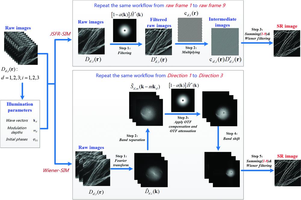
Fig. 1. The workflow of JSFR-SIM is simpler than that of Wiener-SIM. Nine raw images are processed by two distinct workflows to generate a background-free SR image. Top, the simple workflow of JSFR-SIM is predominantly executed in the spatial domain. Bottom, five steps of the conventional Wiener-SIM are executed in Fourier space. Details of each processing approach are presented in Fig. S2 in the Supplemental Materials.

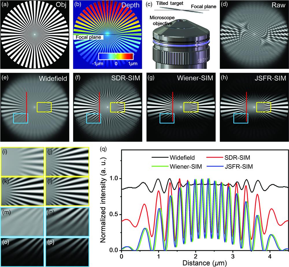
Fig. 2. Simulative results demonstrate the imaging performance of JSFR-SIM. (a) The simulative object is composed of a slightly tilted resolution target. The top and the bottom parts of the target are respectively located 1μm above and below the focal plane, and the middle part of the target is just located at the focal plane, which therefore presents an overall thickness of ∼2μm for the microscope. (b) The depth map of the simulative target. (c) 3D schematic diagram to demonstrate the position of the tilted target. (d) One of the simulated raw images under structured illumination. (e) Wide-field image obtained by summing all raw images. (f) SR image recovered by the SDR-SIM algorithm. Panels (g) and (h) are OS-SR-SIM images restored using Wiener-SIM (with OTF attenuation) and JSFR-SIM, in which the amplitude and the width of the attenuation function are selected as 1.0 and 1.2cycles/μm. Panels (i)–(l) are the close-up views of the yellow-boxed region in (e)–(h), respectively. Panels (m)–(p) are the close-up view of the blue-boxed region in (e)–(h), respectively. (q) The intensity profiles of (e)–(h) along the red solid lines. The numerical aperture of the objective, the wavelength of light, and the pixel size at the focal plane in the simulation were respectively set as 1.49μm, 0.52μm, and 21.6 nm.

Fig. 3. The resolution enhancement of JSFR-SIM is identical to that of Wiener-SIM. (a) Images of 40 nm diameter fluorescent beads captured using widefield microscopy and separately, JSFR-SIM. (b) The close-up view of the widefield and OS-SR-SIM images recovered with JSFR-SIM and Wiener-SIM, focusing on the yellow-boxed region in (a). (c) The xy and the xz cross-sectioned images of an isolated fluorescent bead imaged using widefield, JSFR-SIM, and Wiener-SIM, respectively. Panels (d) and (e) are the intensity profiles of the fluorescent bead along the x- and z-axes imaging using different modalities. Scale bars: (a) 2μm; (b), (c) 500 nm.

Fig. 4. JSFR-SIM enables superior SR imaging of the microtubule cytoskeleton. Microtubules were labeled with GFP as described in Supplementary Note 4 in the Supplemental Materials. The rendered 3D view of the whole cytoskeleton recovered with JSFR-SIM is presented in Video 1. (a) The front-view, left-view, and bottom-view of the rendered 3D image in Video 1. Panels (b)–(d) are, respectively, widefield images and OS-SR-SIM images reconstructed with JSFR-SIM and Wiener-SIM of the specimen at four equidistant focal planes in the white boxed region of (a). (e) The maximum-intensity-projection (MIP) images of the cytoskeleton imaged separately using widefield and JSFR-SIM. The MIP images for each were calculated by projecting the voxels with maximum intensity along the axial direction. Panels (f) and (g) are the close-up views of the widefield, JSFR-SIM, and Wiener-SIM images corresponding to the yellow- and blue-boxed region in (e), respectively. (h) The intensity profiles of the yellow lines in the close-up views in (g). Scale bars: (a)–(d), 10μm; (e) 5μm; (f), (g) 2μm (Video 1, AVI, 7.5 MB [URL: https://doi.org/10.1117/1.AP.4.2.026003.1]; Video 2, AVI, 13.6 MB [URL: https://doi.org/10.1117/1.AP.4.2.026003.2]).

Fig. 5. JSFR-SIM enables clear visualization of microtubule dynamics. Microtubules were labeled with GFP as described in Supplementary Note 4 in the Supplemental Materials. (a) and (b) The first frame of the widefield and OS-SR-SIM movies of the cytoskeleton (Video 3). (c) The close-up view of the time course corresponding to the white-boxed region in (b). The brightness of the series has been normalized to compensate for the photobleaching effect. Blue arrows, one microtubule intersection; yellow arrows, microtubule disassembly event. (d) The close-up view of the time series corresponding to the yellow-boxed region in (b). The red arrows denote a long-duration microtubule assembly event. Panel (e) illustrates the assembly velocity of the microtubule tip as a function of time. Scale bar: (a), (b) 5μm; (c), (d) 2μm (Video 3, AVI, 5.0 MB [URL: https://doi.org/10.1117/1.AP.4.2.026003.3]).

Fig. 6. JSFR-SIM enables near real-time imaging of mitochondrial cristae dynamics and mitochondrial tubulation dynamics. Mitochondria were stained as described in Supplementary Note 4 in the Supplemental Materials. Panels (a) (Video 4) and (d) are the first frames of two different time series, which were both obtained using widefield microscopy and JSFR-SIM, respectively. The solid boxed regions in (a) and (d) are magnified and presented by the time-lapse montages (b), (c), and (e). Yellow arrows in (b) and (e) denote the mitochondrial tubulation event, while the blue arrows in (c) indicate the inter-cristae merging event in which two contiguous cristae structures gradually converge into a single structure. The brightness of the series has been renormalized to compensate for the photobleaching effect. Scale bar: (a), (d) 5μm; (b), (c), (e) 2μm (Video 4, AVI, 6.7 MB [URL: https://doi.org/10.1117/1.AP.4.2.026003.4]).

Table 1. The JSFR-SIM assisted by GPU provides a near-instant reconstruction of all image sizes.