3D shape reconstruction of parabolic trough collector from gradient data based on slope stitching approach

Yinlong Hou; Lin Li; Shanshan Wang; Qiudong Zhu

doi:10.3788/COL201715.111203

Abstract

A method based on slope stitching for measurement of a large off-axis parabolic trough collector is proposed and applied to the surface shape reconstructed from the gradient data acquired by using the reverse Hartmann test. The entire reflector is divided into three sections with overlapping zones along the concentration direction. A mathematical model for the slope stitching algorithm is developed. An improved reconstruction method combining Zernike slope polynomials iterative fitting with the Southwell integration algorithm is utilized to recover the real three-dimensional (3D) shape of the collector. The efficiency and validity of the improved reconstruction method and the stitching algorithm are experimentally verified.

Parabolic trough collectors (PTCs) are widely used in concentrating solar technologies to reflect sunlight onto a specific receiver. In order to reach high optical concentration efficiency values, the geometry, especially the slope, of the reflector surface must be precise. Therefore, it is significant to accurately test and evaluate the geometric precision of the collectors. A variety of techniques have been developed to analyze the surface errors, of which four typical types are video scanning Hartmann optical test (VSHOT)^[1], photogrammetry^[2,3], null-screen testing^[4,5], and deflectometry^[6,7]. However, these measurement techniques cannot simultaneously meet the requirements of accurate, fast, inexpensive, and insensitivity to environmental turbulence at the same time. The setup of photogrammetry and VSHOT is time consuming, and the spatial resolution is limited due to the detection principle. The null-screen testing method and deflectometry is useful for measuring a large parabolic collector^[8–10], and it also can greatly cut down the measurement time. However, for null-screen testing, the design and alignment of the null screens are not easy^[5]. A projector should be used to project stripe patterns on a white target surface, and these patterns also need to be corrected by using deflectometry^[11]. Additionally, the surface shape reconstruction is a trouble in practical measurement. It seems not that easy to obtain very accurate measurement results, as only second-order polynomials may be used to retrieve the surface shape^[12].

In this study, the reverse Hartmann test approach, which can be seen as a combination of deflectometry and VSHOT in some aspects, is used to measure the surface gradient of the PTC. An improved three-dimensional (3D) shape reconstruction method, combining Zernike slope polynomials iterative fitting with the Southwell integration algorithm, is employed in our measurement system for collector shape retrieval. It is well-known that several surface shape detection techniques are based on the measurement of the gradient data, for example, the Hartmann and Shack–Hartmann sensors^[13], the shearing interferometer, Foucault’s knife-edge test, and many others^[14–17]. All of these techniques provide the gradient data of the wavefront or surface. The proposed improved reconstruction algorithm can also be used to retrieve the surface shape or the wavefront. As the test collector is thousands of millimeters in our measurement, the slope stitching technique for connecting separately measured regions is utilized to ensure that the retrieved surface is continuous and smooth.

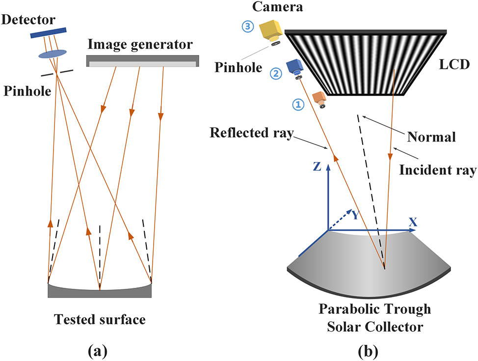
The principle of the reverse Hartmann test method can be described from the point of view of a Hartmann test with the light going through the measurement system in reverse^[18,19], as shown in Fig. 1(a). A liquid crystal display (LCD) is used as the Hartmann stop to display sinusoidal fringe patterns. A detector is used to record the deformed fringes related to surface deviations. A pinhole, which is optimized to limit the width of each reflected beam entering the optical system, is placed in front of the camera. Figure 1(b) shows the schematic diagram of the basic geometric principle that we use for measuring the off-axis parabolic solar mirror with apertures of $1628 mm \times 1700 mm$ .

Sign up for Chinese Optics Letters TOC. Get the latest issue of Chinese Optics Letters delivered right to you！Sign up now

Figure 1.(a) Principle of the reverse Hartmann test. (b) The measurement schematic of the PTC surface.

As shown in Fig. 1(b), the light ray, which is emitted from an LCD and reflected by the measured surface, is collected by the pinhole camera. The angular bisector of the incident ray and the reflected ray is normal to the reflection point on the reflector. The slope at this point can be calculated by measuring the position of the lit pixel on the LCD, the coordinate of pinhole in front of the camera, and the direction vector of the reflected ray. According to the reflection law, the normal $N$ to the surface can be evaluated as $N = \frac{R - I}{| R - I |},$ (1)where $R$ and $I$ are the unit vectors describing the directions of the incident and the reflected rays on the test mirror, respectively, and $N$ is the unit normal vector at the surface.

The reflected ray passes through the pinhole and arrives at the camera image plane. A sixteen-step phase-shifting technique is used, and the light intensity from the LCD screen entering the pinhole camera is $I (x, y) = a + b \cos [ϕ (x, y) + δ],$ (2)where $ϕ (x, y)$ is the phase value to be found, $a$ is the background intensity, $b$ is the amplitude modulation of the patterns, and $δ$ is the additional phase shift $2 π / 16, 4 π / 16, \dots, 32 π / 16$ . Thus, the phase value $ϕ (x, y)$ that represents a unique position on the LCD screen and a CCD detector can be calculated as in Eq. (2): $ϕ (x, y) = \arctan [- \frac{\sum_{i = 1}^{16} I_{i} (x, y) \sin (i \frac{2 π}{16})}{\sum_{i = 1}^{16} I_{i} (x, y) \cos (i \frac{2 π}{16})}] .$ (3)

The absolute phase value can be obtained by using the phase-unwrapping algorithm. The absolute phase of a CCD pixel is equal to the absolute phase of its correspondence point located on the LCD screen. The slopes of a series of corresponding measured points can be obtained by using the reflection law, as the computer-aided design (CAD) model of the solar concentrator can supply an initial estimate of the surface shape. Then, the surface shape can be reconstructed through Zernike slope polynomials iterative fitting and Southwell integration.

A major challenge in optical characterization evaluation of PTC is to detect defects of microns on the surface of thousands of millimeters. The stitching technique based on the reverse Hartmann test is considered to be a practical and efficient method. The measurement of PTC in the $y$ direction can be regarded as the detection of the plane surface, as its curvature is zero. The entire solar concentrator is divided into different regions with overlapping zones. Each region is measured using the reverse Hartmann test, which is scanned over the entire surface. Figure 2 shows the stitching measurement of the PTC in the $y$ direction. In the measurement system, an 80 in. LCD screen is selected to display sinusoidal fringe patterns, which can illuminate the entire test surface. The length of the LCD screen is slightly longer than the length of the PTC in the $y$ direction. According to the reverse Hartmann test principle, half of the cylindrical surface in the $y$ direction can be measured when using only one camera, as shown in Fig. 2(a). Theoretically, two cameras localized at opposite sides of the LCD are enough to collect the entire surface shape data, as shown in Fig. 2(b). As the focal length of the PTC is 1710 mm, the LCD screen can be placed at about the center of the radius of the curvature of the collector. In order to accurately test the geometric precision of the PTC, the CCD plane and the reflector should be conjugate. Thus, the focal length of the lenses used in the pinhole cameras, the field of view, and the angle of inclination of the cameras can be calculated in our measurement system. However, the difficulty lies in obtaining a complete and accurate surface shape for only using two cameras. The overlapping zones are substantially close to zero when using two cameras. In order to effectively use the CCD plane and improve the measurement resolution, eccentric lenses need to be used in the data acquisition systems. In our measurement system, three cameras are used for ensuring measurement accuracy and increasing the slope measurement range of the PTC in the $y$ direction, as shown in Fig. 2(c). Figure 2(d) shows the measurement schematic of the PTC surface along the $y$ axis.

Figure 2.Measurement of the PTC along the $y$ direction. (a) One camera for half of the cylindrical surface, (b) two cameras for the entire cylindrical surface with small overlapping zones, (c) three cameras for the entire cylindrical surface with sufficient overlapping zones, and (d) the measurement schematic of the PTC surface along the $y$ axis.

The problem is then reduced to fitting these three separate measurement regions, which may contain different amounts of piston, tilt, and defocus, back into a complete map of the large off-axis parabolic solar reflector. The slope at discrete points on the test mirror corresponding to each camera can be calculated by using the reverse Hartmann test method. Slope stitching technology has been used to connect the slope values of separately measured regions in the overlapping area. Since the measurements are taken by different cameras, an equally spaced interpolation performed by the use of linearity must be adopted in the overlapping area of two adjacent images. Figure 3 shows the acquisition sections of three cameras corresponding to Fig. 1(b) or Fig. 2(d). The spacing between adjacent sample points is 1 mm. Corresponding to the same point on the test mirror collected by adjacent cameras, its slope value cannot be simply equal to half the sum of the slope values calculated in different acquisition system, as given in Eq. (4). If this calculation method is adopted, there would be obvious stitching traces in the reconstructed surface shape. In this Letter, the weighted average of gradient values in the overlapping region is utilized to stitch these three separate sections together [see Eq. (5)]: ${\begin{cases} S_{12} (x, y) = \frac{C_{1} (m - l + x, y) + C_{2} (x, y)}{2} \\ S_{23} (x, y) = \frac{C_{2} (m - l + x, y) + C_{3} (x, y)}{2} \end{cases} for {\begin{matrix} x = 1, 2, \dots, l \\ y = 1, 2, \dots, n \end{matrix},$ (4) ${\begin{cases} S_{12} (x, y) = \frac{l - x + 1}{1 + l} \cdot C_{1} (m - l + x, y) + \frac{x}{1 + l} \cdot C_{2} (x, y) \\ S_{23} (x, y) = \frac{l - x + 1}{1 + l} \cdot C_{2} (m - l + x, y) + \frac{x}{1 + l} \cdot C_{3} (x, y) \end{cases} .$ (5)

Figure 3.Slope stitching configuration for acquisition sections of three cameras.

In these equations, $S_{12} (x, y)$ and $S_{23} (x, y)$ are the slope values in the $x$ and $y$ directions at the sample points of the overlapping areas; $C_{1} (x, y)$ , $C_{2} (x, y)$ , and $C_{3} (x, y)$ are the slope values of the sample points corresponding to the three cameras. For any arbitrary sample point $P$ lying in the overlapping zone between adjacent subapertures, as shown in Fig. 3, its slope value can be calculated by using Eq. (5) [ $C_{1 P}$ ( $m - l + x, y$ ) for Camera1, $C_{2 P} (x, y)$ for Camera2]. In this way, the slopes of a discrete set of points in the common area of the overlapping zone can be obtained. Then, the overall surface shape of the PTC can be reconstructed by Zernike slope polynomials iterative fitting, as the surface retrieval is useful for improving the manufacturing and installing process, and all of the slope values are analyzed to determine the expansion coefficients, as described in detail in the subsequent section. The retrieved surface is continuous and smooth by using slope stitching technology.

It is well-known that the terms of orthonormal Zernike polynomials associate with different types of aberrations. It is convenient to express the reflector shape by a linear combination of Zernike polynomials, as the removing of tilts and defocusing is simple. The expansion of the function can be written as $W (x, y) = \sum_{i = 0}^{N} C_{i} Z_{i} (x, y),$ (6)where $W (x, y)$ is the surface shape function, $C_{i}$ is the expansion coefficients to be determined, and $Z_{i}$ ( $x$ , $y$ ) is the Zernike polynomials. The gradient data of the estimation formula can be expressed by differentiating Eq. (6): ${\begin{matrix} \frac{\partial W (x, y)}{\partial x} = \sum_{i = 0}^{N} C_{i} \frac{\partial Z_{i} (x, y)}{\partial x} \\ \frac{\partial W (x, y)}{\partial y} = \sum_{i = 0}^{N} C_{i} \frac{\partial Z_{i} (x, y)}{\partial y} \end{matrix} .$ (7)

Equation (7) can be given in matrix form: $S = P * C,$ (8)where $S$ is the vector that contains all of the measured slope values ( $\partial W / \partial x, \partial W / \partial y$ ), $P$ is the partial differential Zernike polynomials matrix ( $\partial Z_{i} / \partial x, \partial Z_{i} / \partial y$ ), and $C$ is the column vector containing terms of $C_{1}, C_{2}, \dots$ , and $C_{N}$ . The unknown expansion coefficients $C_{i}$ can be calculated by using the standard least-squares fitting. Then, substituting $C_{i}$ into Eq. (6), the tested reflector shape can be reconstructed. Theoretically, the process of 3D shape retrieval is ideal because the unit normal vectors $N$ accurately are known. In practice, the collector deformations can achieve the millimeters level, and the gradient data may not be ideally available for the entire surface as expected. In order to reconstruct the 3D shape of the PTC with desired accuracy, successive Zernike slope polynomials iterations is employed. Figure 4 illustrates the iterative algorithm. The implementation details of the iterative process can be described in the following steps: Step 1: Substitute the designed value of the surface shape for initial iteration value. Express the designed collector in terms of Zernike polynomials by Eq. (6) and least-squares fitting. Set the iterative number as $j = 1$ .Step 2: Calculate the gradient data of each sampling point by Eq. (1), as the direction vectors corresponding to different pixels in the CCD plane can be obtained by using the calibration technique. Update $j = j + 1$ .Step 3: Take slope Zernike polynomials fitting according to Eqs. (7)–(8) and standard least-squares fitting to estimate $C^{(j)}$ . Substitute $C^{(j)}$ into Eq. (6) to obtain the 3D shape of the collector $W^{(j)}$ .Step 4: Check the difference between the updated surface estimation and the previous estimation. If the 3D shape differences are $| W^{(j)} - W^{(j - 1)} | \geq 10^{- 6} mm$ recalculate the slope values and go back to Step 2. Otherwise, end the loop.Step 5: Iterative terminate, recover the 3D surface shape of the PTC.

The Zernike slope polynomials iterative fitting technique provides the overall surface shape of the large reflector. The iterative process can also guarantee the stability and robustness in practical measurement. However, localized or small errors will not appear in the final polynomial fit, as only a limited number of terms are used. In order to retrieve the high frequency information of the surface shape, Southwell integration is made on the basis of iterations of Zernike slope polynomials. The relations of the height difference and the slope can be presented by ${\begin{matrix} (h_{m + 1, n} - h_{m, n}) \cdot Δ = (s_{m + 1, n}^{x} + s_{m, n}^{x}) / 2 = s_{m + 1 / 2, n}^{x} \\ (h_{m, n + 1} - h_{m, n}) \cdot Δ = (s_{m, n + 1}^{y} + s_{m, n}^{y}) / 2 = s_{m, n + 1 / 2}^{y} \end{matrix},$ (9)where $h_{m, n}$ represents the surface height at certain point ( $m$ , $n$ ) in a sample point array of $M$ columns by $N$ rows. $1 / Δ$ is the sample spacing between two adjacent points, $s_{m, n}^{x}$ and $s_{m, n}^{y}$ are the slope values in the $x$ and $y$ directions. $(M - 1) \times N$ equations along the horizontal direction and $M \times (N - 1)$ equations along the vertical direction [like Eq. (9)] can be obtained as illustrated in Fig. 5. The $3 \times 3$ points are used to represent $M \times N$ sample points, the slope values $s_{1}$ to $s_{6}$ and $s_{7}$ to $s_{12}$ are used to replace $s_{m + 1 / 2, n}^{x}$ and $s_{m, n + 1 / 2}^{y}$ , which are half of the slopes of two adjacent points. Thus, a set of equations relating slopes to the surface heights can be expressed as the right side in Fig. 5. In order to calculate the surface heights of these sample points, the means of a least-squares algorithm can be used. In the process of surface retrieval, we substitute slope deviations between the actual slope values and differential values of Zernike polynomials iteration surface shape for slopes $s_{m, n}$ . Surface deformations from the iteration surface shape can be obtained by Southwell integration, which contains high frequency errors. In our 3D shape reconstruction algorithm, the Zernike slope polynomials iterative fitting result is set to be the initial value of the Southwell integration method.

Figure 4.Iterative process for 3D shape reconstruction of the collector.

Figure 5.Southwell integration for surface shape reconstruction.

The schematic of the reverse Hartmann layout for scanning and measuring the large off-axis parabolic solar collector (focal length of 1710 mm) is shown in Fig. 6. The test reflector is adjusted by a platform, which consists of a granite platform used as the base plane, four well-thought-out support structures used to mount the concentrator, and four pillars to position the PTC. An 80 in. LCD screen configured at a resolution of $1080 \times 1920 pixels$ was used to generate sixteen-step phase-shifting fringe patterns. Three pinhole CCD cameras with the pixel pitch of 5.2 μm were setup next to the LCD to receive the reflected deformed fringe patterns. According to the curvature radius and shape of the collector, the relative position of the LCD, PTC, and pinhole cameras can be optimized. The pinhole cameras and LCD screen were 4612.6 and 4629.3 mm away from the platform in the $z$ direction, respectively. The distance between the two edges of the collector and the platform were both 394.9 mm. The field of view of each pinhole camera is about 11.5°. Horizontal and vertical fringes were projected onto the LCD screen, and the deformed fringes were synchronously recorded by three cameras. The 3D shapes were precisely reconstructed by Zernike slope polynomials iterative fitting and Southwell integration for low to middle frequency information and high frequency information of the PTC, respectively.

Figure 6.Schematic of the experiment setup for using the reverse Hartmann test to measure the large collector.

The measured slope deviations for each camera are shown in Figs. 7(a) and 7(b) [(a1)–(a3) correspond to the $x$ direction, (b1)–(b3) correspond to the $y$ direction]. The sizes of these three subapertures are $1628 mm \times 624 mm$ , $1628 mm \times 848 mm$ , and $1628 mm \times 572 mm$ , respectively. An overlapping of 20% is maintained. All three sections are stitched together by utilizing the slope stitching approach. The stitched mathematical model is experimentally verified. Figures 7(c1)–7(c2) present the stitched slope deviations. The piston, tilt, defocus, and other primary Zernike aberrations are subtracted in these deviation maps. The red and blue colors in the images represent the magnitude of deviations, which is up to $+ 11$ and $- 11 mrad$ . Figure 7(c3) shows the collector deformation shape (low-order shape removed) from the slope polynomial fitting and integration with the Zernike iteration and Southwell zonal methods. The high frequency surface shape information is especially useful for improving the collector fabrication and installation process. Figures 7(d1)–7(d3) present the calculated gradient data and reconstructed 3D shape of the PTC.

Figure 7.(a) Experimentally measured slope deviations for three cameras on the $x$ axis, (b) experimentally measured slope deviations for three cameras on the $y$ axis, (c) stitched gradient data and height deformation, and (d) slope distributions and 3D shape of the PTC.

In conclusion, we present a metrology scheme for the surface measurement and shape reconstruction of a parabolic trough solar collector by a slope stitching technique using the reverse Hartmann test. A mathematical model for slope stitching of the large off-axis reflector is developed. An improved reconstruction algorithm, incorporating Zernike slope polynomials iterative fitting and the Southwell integration algorithm, is utilized to reconstruct the surface shape from gradient data in a rectangular-shaped aperture. The iterative process based on the Zernike slope polynomials fitting technique can guarantee the robustness and stability in practical measurement. Southwell integration based on the iterations is employed to calculate the high frequency information of the collector. The stitching technique and the reconstruction algorithm are verified by performing the experimental studies on the large collector. The proposed method is a stable, efficient, accurate, and cost-effective approach to solve the 3D shape reconstruction problem of a large parabolic trough solar collector from the measured gradient data acquired by the reverse Hartmann test.

References

[1] S. A. Jones, J. K. Gruetzner, R. M. Houser, R. M. Edgar, T. J. Wendelin. Proceedings of the 32nd Intersociety Energy Conversion Engineering Conference, 1997. IECEC-97, 1877(1997).

[2] M. R. Shortis, G. H. G. Johnston. J. Solar Energy Eng. Trans. ASME, 118, 146(1996).

[3] K. Pottler, E. Lupfert, G. H. G. Johnston, M. R. Shortis. J. Solar Energy Eng. Trans. ASME, 127, 94(2005).

[4] V. I. Moreno-Oliva, M. Campos-Garcia, E. Roman-Hernandez, A. Santiago-Alvarado. Opt. Eng., 53, 114108(2014).

[5] V. I. Moreno Oliva, R. Uribe, M. Campos-García. Solar Collectors and Panels, Theory and Applications(2010).

[6] M. C. Knauer, J. Kaminski, G. Hausler. Proc. SPIE, 5457, 366(2004).

[7] S. Ulmer, T. Maerz, C. Prahl, W. Reinalter, B. Belhomme. Solar Energy, 85, 681(2011).

[8] M. Avendaño-Alejo, V. I. Moreno-Oliva, M. Campos-García, R. Díaz-Uribe. Appl. Opt., 48, 1008(2009).

[9] M. Campos-Garcia, V. I. Moreno-Oliva, R. Diaz-Uribe, F. Granados-Agustin, A. Santiago-Alvarado. Appl. Opt., 50, 3101(2011).

[10] F. Patio-Jimenez, Y. Nahmad-Molinari, V. I. Moreno-Oliva, F. D. L. Santos-Garcia, A. Santiago-Alvarado. Int. J. Photoenergy, 2015, 196186(2015).

[11] T. Maerz, C. Prahl, S. Ulmer, S. Wilbert, C. Weber. J. Solar Energy Eng. Trans. ASME, 133, 31022(2011).

[12] M. I. Pena-Cruz, C. A. Arancibia-Bulnes, A. M. Vidal, M. S. Gonzalez. J. Renewable Sustainable Energy, 6, 013118(2014).

[13] L. Yang, L. Hu, D. Li, Z. Cao, Q. Mu, J. Ma, L. Xuan. Chin. Opt. Lett., 13, 120801(2015).

[14] D. Malacara. Optical Shop Testing(2007).

[15] H. Cui, W. Liao, N. Dai, X. Cheng. Chin. Opt. Lett., 10, 031201(2012).

[16] F. Zhou, X. Chen, H. Tan, X. Chai. Chin. Opt. Lett., 14, 111403(2016).

[17] K. Liu, C. Zhou, S. Wang, S. Wei, X. Fan. Chin. Opt. Lett., 13, 081101(2015).

[18] P. Su, R. E. Parks, L. R. Wang, R. P. Angel, J. H. Burge. Appl. Opt., 49, 4404(2010).

[19] E. Kewei, L. Dahai, L. Mengyang, Z. Jiwen, L. Shuiyan, Z. Chong, D. Zhenqiang, W. Qionghua. Acta Opt. Sin., 34, 112004(2014).