
M. Zitelli, M. Ferraro, F. Mangini, S. Wabnitz. Single-mode spatiotemporal soliton attractor in multimode GRIN fibers[J]. Photonics Research, 2021, 9(5): 741
- Photonics Research
- Vol. 9, Issue 5, 741 (2021)
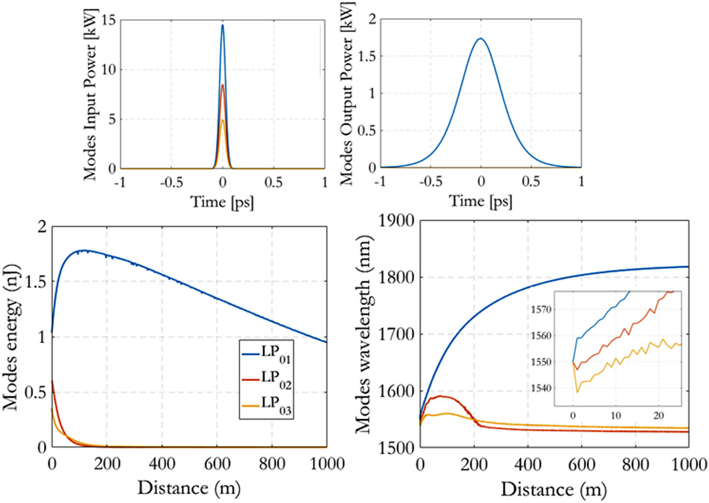
Fig. 1. Simulated energy and wavelength evolution of the three input axial modes. The two upper insets show the pulse power modal distribution at the input (left), and after 1 km of propagation (right).
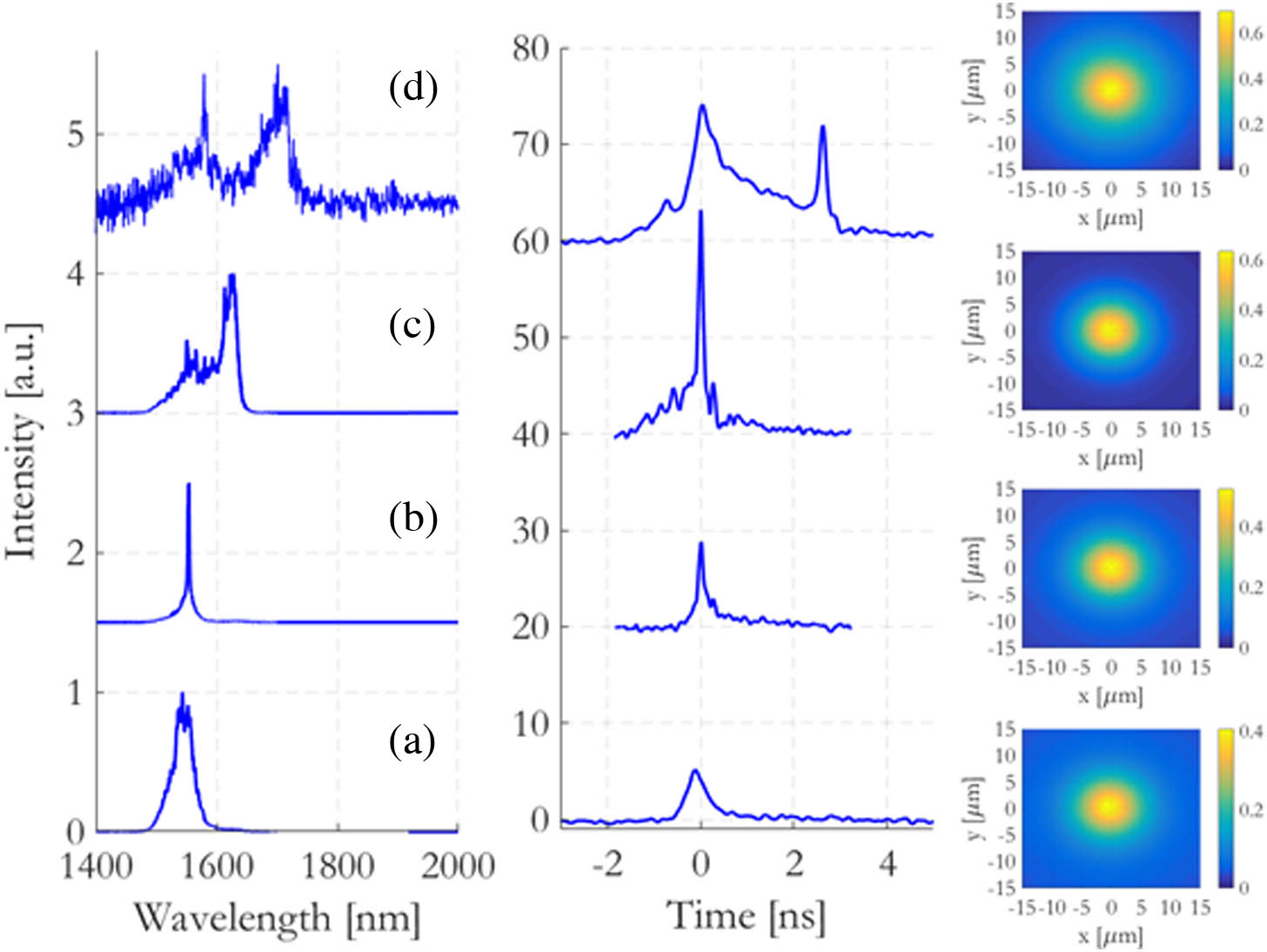
Fig. 2. Measured output spectra (left column), photodiode traces (center column), and near-field (right column) at 1 km distance, for input pulse peak powers of (a) 2 kW, (b) 6.4 kW, (c) 15 kW, and (d) 110 kW (see Visualization 1 ).
Fig. 3. Top: Measured wavelength for the three generated solitons versus input peak power. Bottom: corresponding soliton bandwidth evolution.
Fig. 4. Measured beam waist at 1 km distance versus input peak power, when the input beam is coupled with 0°, 2.3°, and 4.6° tilt angle, as compared with the theoretical fundamental mode waist. Input beam waist is 15 μm. Insets show measured output beam shapes at powers indicated by the arrows.
Fig. 5. Measured and simulated FWHM pulse width at 120 m distance versus input peak power. The top insets are autocorrelation traces at 21 kW, 28 kW, and 109 kW input power, respectively.
Fig. 6. Measured bandwidth versus input peak power, for the two solitons observed after 120 m of GRIN fiber.
Fig. 7. Near-field beam waist versus input peak power, for the first soliton at 120 m of GRIN fiber length.
Fig. 8. Recorded autocorrelation traces (left column) and near-field beams (right column) from 120 m of GRIN fiber, for input peak powers: (a) 22 kW, (b) 29 kW, (c) 37 kW, and (d) 109 kW.

Set citation alerts for the article
Please enter your email address
© Copyright 2018-2021 | Chinese Laser Press. All Rights Reserved 沪ICP备15018463号-20