Improved modulation format identification based on Stokes parameters using combination of fuzzy c-means and hierarchical clustering in coherent optical communication system

Longxue Cheng; Lixia Xi; Donghe Zhao; Xianfeng Tang; Wenbo Zhang; Xiaoguang Zhang

doi:10.3788/COL201513.100604

Abstract

In this Letter, we develop the Stokes space-based method for modulation format identification by combing power spectral density and a cluster analysis to identify quadrature amplitude modulation (QAM) and phase-shift keying (PSK) signals. Fuzzy c-means and hierarchical clustering algorithms are used for the cluster analysis. Simulations are conducted for binary PSK, quadrature PSK, 8PSK, 16-QAM, and 32-QAM signals. The results demonstrate that the proposed technique can effectively classify all these modulation formats, and that the method is superior in lowering the threshold of the optical signal-to-noise ratio. Meanwhile, the proposed method is insensitive to phase offset and laser phase noise.

The continued demand for increased optical network capacities provides challenges for current and future network designs. To overcome these challenges, elastic optical networks equipped with flexible transceivers are required^[1]. In order to demodulate signals optimally at the receiver side^[2], modulation format identification (MFI) is needed in future elastic optical networks.

Exploration for MFI techniques in optical communication has just begun. Four different methods have been employed for optical MFI: (a) identification from constellation diagrams using k-means, which is simple but requires a carrier and phase recovery before MFI^[3]; (b) artificial neural network-based identification, which can recognize all the formats but needs prior training^[4]; (c) principal component analysis-based pattern recognition on asynchronous delay-tap plots, which can realize channel estimation in the meantime but needs specific amounts of sampling points^[5]; (d) the Stokes space and machine learning technique^[6].

Here, we theoretically analyze the distribution characteristics of Stokes space clusters for different formats. Based on this, Stokes parameters are extracted in the coherent receiver and utilized to distinguish between quadrature amplitude modulation (QAM) and phase-shift keying (PSK) signals. Furthermore, a decision criterion combining fuzzy c-means (FCM) and a hierarchical clustering algorithm is used to provide enhanced discrimination among the modulation formats. This method was proved applicable to wireless communications^[7]. The identification algorithm is implemented after chromatic dispersion (CD) compensation.

Sign up for Chinese Optics Letters TOC. Get the latest issue of Chinese Optics Letters delivered right to you！Sign up now

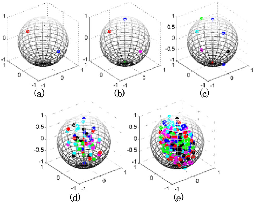
For polarization-multiplexed (PM) system, the received signal $R$ can be expressed with the Jones vector in the following form: $R = [\begin{array}{l} E_{x} \\ E_{y} \end{array}] = [\begin{array}{l} A_{x} e^{j φ_{x}} \\ A_{y} e^{j φ_{y}} \end{array}] .$ (1)

The Jones vector is transformed into the Stokes vector, $S$ , as follows^[8]: $S = [\begin{array}{l} s_{0} \\ s_{1} \\ s_{2} \\ s_{3} \end{array}] = [\begin{array}{l} A_{x}^{2} + A_{y}^{2} \\ A_{x}^{2} - A_{y}^{2} \\ 2 A_{x} A_{y} \cos δ \\ 2 A_{x} A_{y} \sin δ \end{array}],$ (2)where $δ = φ_{x} - φ_{y}$ is the phase difference between the $X$ and $Y$ polarization components of the Jones vector $R$ . If the frequency offset, laser linewidth, and initial phase are considered in the received signal, they just change the phase of $E_{x}$ and $E_{y}$ , and hence the Stokes parameters are not affected, as shown in Eq. (2). Thus, the proposed method is insensitive to these impairments. When normalized by $\max (s_{0})$ , the vector ${[\bar{s_{1}}, \bar{s_{2}}, \bar{s_{3}}]}^{T}$ indicates different points inside the Poincaré sphere. Different modulation formats exhibit different signatures in accordance with the number of clusters inside the Poincaré sphere; therefore, we can identify modulation formats by recording the number of clusters. For binary PSK (BPSK), quadrature PSK (QPSK), 8PSK, 16-QAM, and 32-QAM signals, the numbers of clusters are 2, 4, 8, 60, 248, and the distributions inside the Poincaré sphere are shown in Fig. 1.

Figure 1.Stokes cluster inside the Poincaré sphere. (a) PM-BPSK, (b) PM-QPSK, (c) PM-8PSK, (d) PM-16-QAM, and (e) PM-32-QAM.

We theoretically derived the distributions for different modulation formats. Take 16-QAM, for example: the distribution of clusters is derived as follows.

Figure 2 shows the constellation diagram of 16-QAM, and the possible values of amplitude $A$ and phase $φ$ are listed in Table 1.

Figure 2.Constellation diagram of 16-QAM.

Amplitude (Ax or Ay)	Phase (φx or φy)
2	±π4,±3π4
10	±π10,±4π10,±6π10,±9π10
32	±π4,±3π4

Table 1. Amplitude and Phase of 16-QAM

View all Tables

The corresponding Stokes vector can be calculated via Eq. (2). The possible values of ${[s_{1}, s_{2}, s_{3}]}^{T}$ are listed in Table 2. The number of clusters of the 16-QAM signal is 60.

(Ax,Ay)	δ	(s1,s2,s3)
(2,2)	0,±π2,π	(0,0,±4),(0,±4,0).
(10,10)	0,±2π10,±3π10,±5π10,±7π10,±8π10,π	(0,0,±20),(0,±20,0), (0,±20 cos 2π10,±20 sin 2π10), (0,±20 cos 3π10,±20 sin 3π10).
(32,32)	0,±π2,π	(0,0,±36),(0,±36,0).
(2,10)	±3π20,±7π20,±13π20,±17π20	(±8,±220 cos 3π20,±220 sin 3π20), (±8,±220 cos 7π20,±220 sin 7π20).
(2,32)	0,±π2,π	(±16,0,±12),(±16,±12,0).
(10,32)	±3π20,±7π20,±13π20,±17π20	(±8,±620 cos 3π20,±620 sin 3π20), (±8,±620 cos 7π20,±620 sin 7π20).

Table 2. Possible Values of (s1,s2,s3)

View all Tables

Figure 1 shows that the number of clusters increases sharply when the order of modulation increases. The distances between clusters become smaller, and distinguishing between the adjacent clusters becomes more difficult. Nevertheless, we find that the data is characterized by symmetry from Table 2. Therefore, the number of clusters whose coordinate values, $s_{1}$ , $s_{2}$ , and $s_{3}$ are all nonnegative can be utilized to distinguish different QAM signals. The corresponding numbers for 16-QAM and 32-QAM are 14 and 43, respectively, which is shown in Fig. 3.

Figure 3.Stokes cluster with nonnegative coordinate values inside the Poincaré sphere. (a) PM-16-QAM and (b) PM-32-QAM.

We first distinguish between the PSK and QAM signals. The key feature used is the maximum value of the power spectral density of the normalized-centered instantaneous amplitude $γ_{\max}$ , which is defined by $γ_{\max} = \max {| DFT (a_{c n} (i)) |}^{2} / N_{s},$ (3)where $N_{s}$ is the number of symbols, DFT means discrete Fourier transform, and $a_{c n} (i)$ is the value of the normalized-centered instantaneous amplitude at the time instants $t = i / f_{s}$ , $i = 1, 2, \dots, N_{s}$ , defined by $a_{c n} (i) = a_{n} (i) - 1 .$ (4)

Here, $a_{n} (i) = a (i) / m_{a}$ , where $m_{a}$ is the average value of the instantaneous amplitude $m_{a} = \frac{1}{N_{s}} \sum_{i = 1}^{N_{s}} a (i) .$ (5)

For ideal PSK signals, there is no amplitude modulated information and $a_{c n} (i)$ is zero; thus, the parameter $γ_{\max}$ is zero theoretically. For QAM signals, the amplitude is not constant and $a_{c n} (i)$ varies; thus, $γ_{\max}$ is much higher than zero^[9]. The PSK and QAM signals can be distinguished by setting an appropriate threshold of $γ_{\max}$ . Additionally, utilizing the spectral power density rather than the time domain data can lower the influence of burst noise.

After distinguishing between the PSK and QAM signals, we combine the FCM algorithm and hierarchical clustering to further identify M-PSK and M-QAM signals.

FCM is the most popular fuzzy-clustering algorithm. It is based on the minimization of the following objective function^[10]: $J_{m} = \sum_{i = 1}^{N} \sum_{j = 1}^{C} u_{i j}^{m} {‖ x_{i} - c_{j} ‖}^{2}, 1 \leq m < \infty,$ (6)where $m$ is an arbitrary real number greater than 1, $N$ is the number of sampling points, and $C$ is the clustering number. $u_{i j}$ stands for the degree of membership for cluster $j$ , $x_{i}$ represents the $i$ th measured data, $c_{j}$ is the $j$ th center of the cluster, and $‖ • ‖$ is the Euclidean distance between any measured data and the center.

Fuzzy partitioning is carried out through an iterative optimization of the objective function in Eq. (6), with the update of membership $u_{i j}$ and the cluster centers $c_{j}$ by $u_{i j} = \frac{1}{\sum_{k = 1}^{C} {(\frac{‖ x_{i} - c_{j} ‖}{‖ x_{i} - c_{k} ‖})}^{\frac{2}{m - 1}}},$ (7) $c_{j} = \frac{\sum_{i = 1}^{N} u_{i j}^{m} \cdot x_{i}}{\sum_{i = 1}^{N} u_{i j}^{m}} .$ (8)

FCM is sensitive to initial conditions, especially the initial cluster centers, which may lead to local minimum results. To avoid the local result, a simple and efficient select rule of the initial cluster centers is applied in the FCM algorithm^[11].

This iteration will stop when $\max_{i j} {| u_{i j}^{(k + 1)} - u_{i j}^{(k)} |} < ε$ is satisfied, where $ε$ is a termination criterion between 0 and 1, and $k$ is number of iteration steps.

After the FCM algorithm iterates over, the number of clusters is constant, which cannot determine the modulation formats. Determining the actual number of clusters is necessary in the next step, which is based on hierarchical clustering, where data is grouped by creating a cluster tree over a variety of scales. The procedure of hierarchical clustering is as follows: first, we calculate the Euclidean distance between every pair of objects in the data set (centroids after FCM clustering). Then, we group the objects into a binary, hierarchical cluster tree. Finally, we determine where to cut the hierarchical tree into clusters, which will achieve different numbers of clusters. The cluster number can be assigned from $1, 2 \dots K$ ( $K$ is the number of clusters in the FCM algorithm). In this step, we calculate the objective function for each possibility, and the number of optimum clusters corresponds to the minimum value of the objective function. The objective function is defined as follows^[12]: $V = \frac{\sum_{i = 1}^{C} \sum_{j = 1}^{N} u_{i j}^{2} {‖ c_{i} - x_{j} ‖}^{2} + \frac{1}{C (C - 1)} \sum_{i = 1}^{C} \sum_{k = 1, k \neq i}^{C} {‖ c_{i} - c_{k} ‖}^{2}}{\min_{i \neq k} {‖ c_{i} - c_{k} ‖}^{2} + \frac{1}{C}} .$ (9)

For every modulation format, a range is set. We propose to use the range where the cluster result (the number of clusters) falls as the decision metrics.

Simulations using VPI and MATLAB are carried out to verify the above method. Figure 4 shows the simulation setup. In the transmitter, 28GBaud PM-BPSK, PM-QPSK, PM-8PSK, PM-16-QAM, and PM-32-QAM signals are generated separately. In the optical channel, the PM signal passes through the optical fiber, the set optical signal-to-noise ratio (OSNR) module, and the polarization mode dispersion (PMD) emulator. After coherent detection and two-fold oversampling, four-channel signals are sent to the digital signal processing module, which is implemented using MATLAB. After CD compensation, MFI is performed. The dotted frame at lower side of Fig. 4 shows the identification flow.

Figure 4.Simulation setup and decision flowchart.

In the first step, the threshold of $γ_{\max}$ is set to 1, which is determined from a number of simulations. The PSK and QAM formats can be successfully identified when the OSNR is above 16 dB. Figure 5 shows the values of $γ_{\max}$ versus different OSNRs for different modulation formats.

Figure 5. $γ_{\max}$ versus OSNR for various modulation formats.

Next, the FCM and hierarchical clustering are combined to further distinguish between the PSK and QAM signals. The decision range for every format is listed in Table 3.

Figure 6 shows the probability of correct identification under the effect of OSNR. The OSNR values for different formats are well chosen based on the needs of a commercial system. As can be seen from Fig. 6, the probability of correct identification increases when the OSNR increases, except for the BPSK signal. Even when the OSNR is as low as 1 dB, the BPSK signals can be identified with 100% probability. For the QPSK, 8PSK, 16-QAM, and 32-QAM signals, the thresholds of identification with 100% probability are 17, 22, 28, and 30 dB.

Figure 6.Probability of correct identification versus OSNR.

	BPSK	QPSK	8PSK	16-QAM	32-QAM
Theoretical Value	2	4	8	14	43
Decision Metric	[1,2]	[4,5]	[7,11]	[12,28]	[29,51]

Table 3. Optimal Cluster Number

View all Tables

Figure 7 shows the probability of correct identification under the effect of the first-order PMD, which is quantified by differential group delay (DGD). Here, we just list the results for the QPSK and 32-QAM signals. The OSNR values are set to 17 and 30 dB independently. As can be seen from Fig. 7, the probability of correct identification decreases as the DGD increases. The thresholds of identification with 100% probability for the QPSK and 32-QAM signals are 22 and 14 ps. So, this method shows high tolerance to first-order PMD.

Figure 7.Probability of correct identification versus DGD.

In conclusion, we improve the Stokes space-based MFI method in Ref. [6] by combing power spectral density and a cluster analysis. The process of clustering utilizes FCM and hierarchical clustering algorithms. The simulation results indicate that the method shows higher tolerance to OSNR and first-order PMD than the method in Ref. [6], and our method is insensitive to the laser linewidth. Meanwhile, we extend the modulation formats that can be identified to 32-QAM signals. Since this method is sensitive to CD, it must be implemented in systems where the CD can be monitored and compensated precisely, like the systems in Refs. [13,14]. Meanwhile, the Stokes-based method only can be used in a receiver capable of measuring Stokes parameters^[6].

References

[1] K. Roberts, C. Laperle. Proceedings of the ECOC, 1(2012).

[2] I. T. Monroy, D. Zibar, N. G. Gonzalez, R. Borkowski. Proceedings of the 13th ICTON, 1(2011).

[3] N. G. Gonzalez, D. Zibar, I. T. Monroy. Proceedings of the ECOC, 6, 11(2010).

[4] F. N. Khan, Y. Zhou, A. P. Lau, C. Lu. Opt. Express, 20, 12422(2012).

[5] M. C. Tan, F. N. Khan, W. H. Al-Arashi, Y. D. Zhou, A. P. T. Lau. J. Opt. Commun. Networking, 6, 441(2014).

[6] R. Borkowski, D. Zibar, A. Caballero, V. Arlunno, I. T. Monroy. Photon. Technol. Lett., 25, 2129(2013).

[7] N. Ahmadi, R. Berangi. Signal Process.: Int. J., 4, 123(2010).

[8] B. Szafraniec, B. Nebendahl, T. Marshall. Opt. Express, 18, 17928(2010).

[9] A. K. Nandi, E. E. Azzouz. Signal Process., 46, 211(1995).

[10] J. C. Bezdek. Pattern Recognition with Fuzzy Objective Function Algoritms(1981).

[11] H. Z. Zhang, J. Wang. OALib J., 36, 206(2009).

[12] Y. Tang, F. Sun, Z. Sun. Proceedings of the American Control Conference, 1120(2005).

[13] Y. Sun, L. Xi, X. Tang, D. Zhao, Y. Qiao, X. Zhang, X. Zhang. Chin. Opt. Lett., 12, 100606(2014).

[14] C. Gao, S. Huang, J. Xiao, X. Gao, Q. Wang, Y. Wei, W. Zhai, W. Xu, W. Gu. Chin. Opt. Lett., 13, 010604(2015).