• Infrared and Laser Engineering
  • Vol. 50, Issue 6, 20200523 (2021)
Xiao Liang1, Huilin Jiang2, Hao Sun1, Chunyan Wang1, and Huan Liu1
Author Affiliations
  • 1School of Opto-Electronic Engineering, Changchun University of Science and Thchnology, Changchun 130022, China
  • 2Institute of Space Photoelectric Technology, Changchun University of Science and Technology, Changchun 130022, China
  • show less
    DOI: 10.3788/IRLA20200523 Cite this Article
    Xiao Liang, Huilin Jiang, Hao Sun, Chunyan Wang, Huan Liu. Solving initial structure of bifocal system according to theory of paraxial optics[J]. Infrared and Laser Engineering, 2021, 50(6): 20200523 Copy Citation Text show less
    Structure diagram of axial bifocal optical system
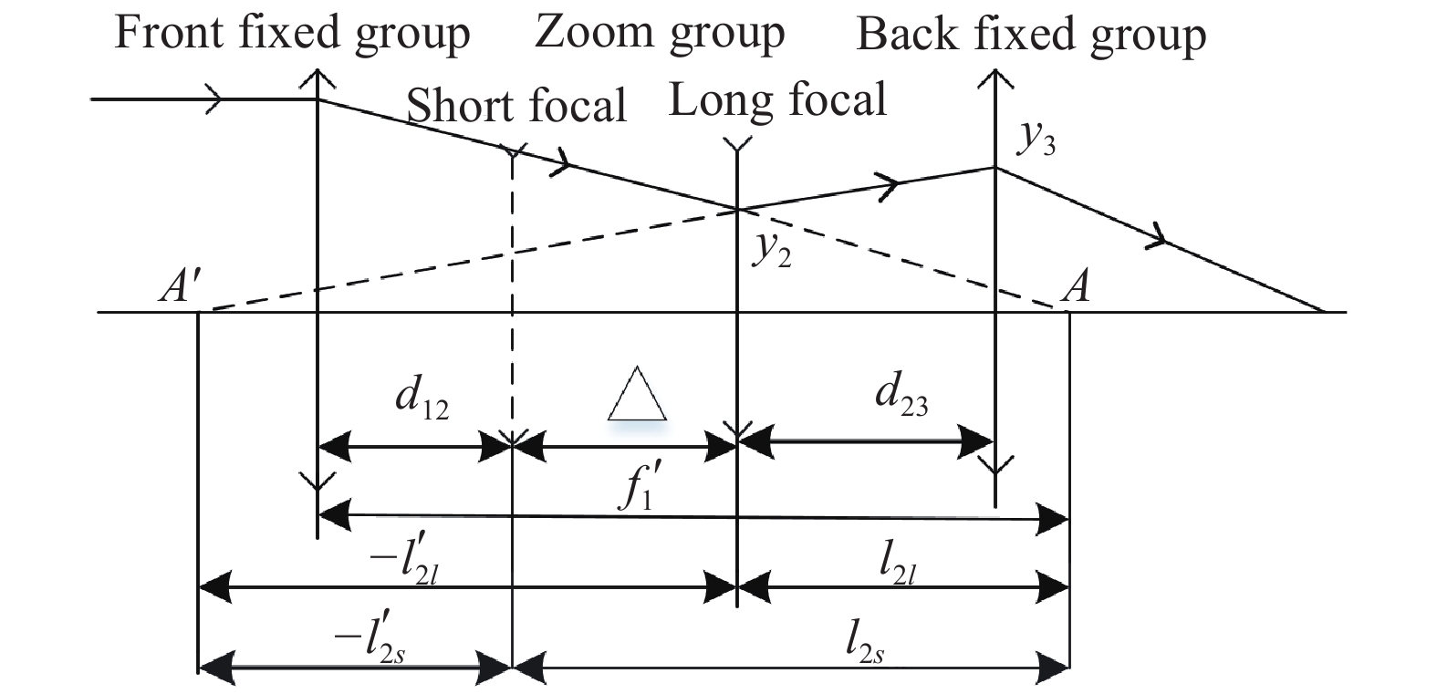
    Fig. 1. Structure diagram of axial bifocal optical system
    Light path of paraxial optical system
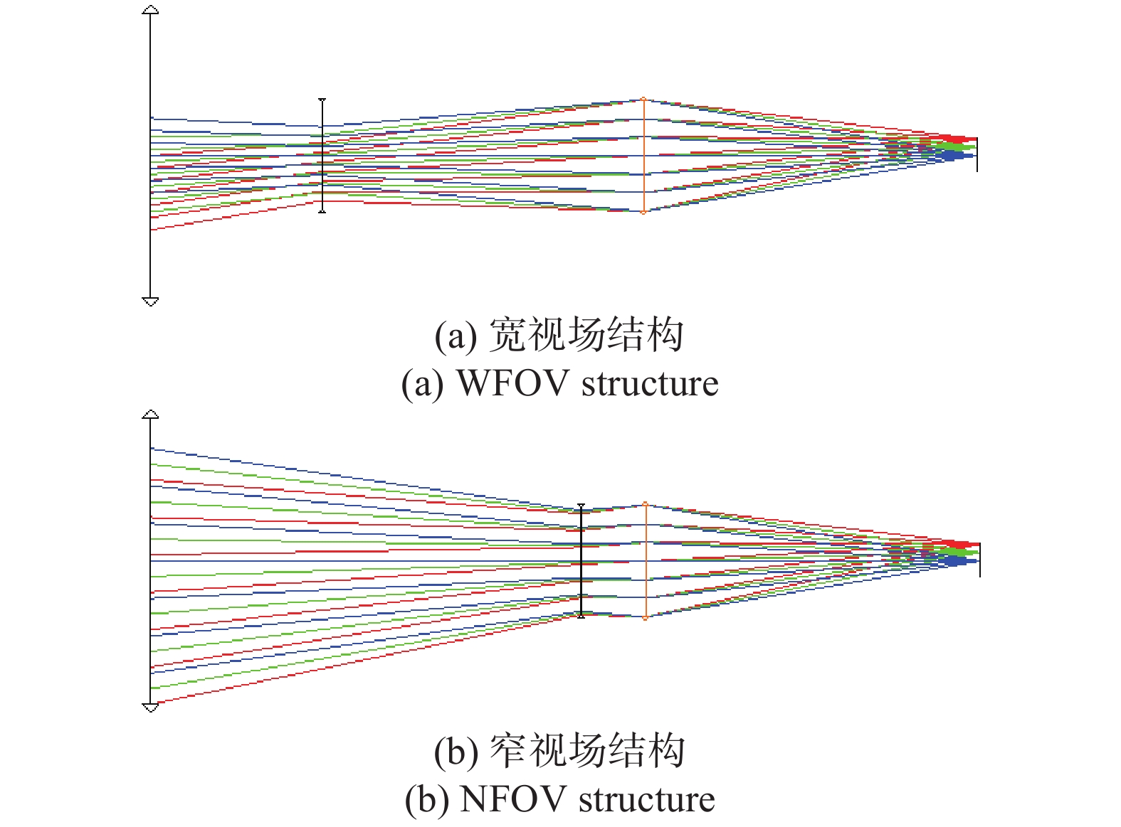
    Fig. 2. Light path of paraxial optical system
    Light path after the first step optimization
    Fig. 3. Light path after the first step optimization
    Light path after the second step optimization
    Fig. 4. Light path after the second step optimization
    Light path diagram after the third step optimization
    Fig. 5. Light path diagram after the third step optimization
    Light path and aberration diagram. (a) Light path; (b) Spot diagram; (c) MTF; (d) Field curvature and distortion; (e) Lateral color
    Fig. 6. Light path and aberration diagram. (a) Light path; (b) Spot diagram; (c) MTF; (d) Field curvature and distortion; (e) Lateral color
    [in Chinese]
    Fig. 6. [in Chinese]
    ParameterValue
    Wavelength486-656 nm
    Field of view8.6°/2.9°
    Focal length40 (WFOV) mm 120 (NFOV) mm
    Spot diagram<0.5 pixel@0-0.707 fields <0.7 pixel@0.707-1 fields
    MTF100 lp/mm>0.3
    Temperature−20-45 ℃
    CCD pixel5 μm
    Table 1. Design index of optical system
    Radius/mmThickness/mmGlass
    75.1834.46Zk13
    −23.1741.063
    −20.4561.977Sf6
    −43.44311.686
    914.6722.267Sk11
    −39.32150.766
    Table 2. Lens parameters after the first step optimization
    Radius/mmThickness/mmGlass
    −53.0121.999P-sf68
    −33.6810.998
    −35.3821.999N-lak33b
    69.94856.318/1.357
    128.8813.276Zk13
    −34.6621.524
    −26.7161.999Sf6
    −60.5430.999
    117.3078.127Sk11
    −44.07864.357
    Table 3. Lens parameters after the second step optimization
    SurfaceRadius/mmThickness/mmGlass
    157.87010Zk12
    2−77.1062Kzfs8
    3193.41913.083/59.282
    4−42.4194.997P-sf68
    5−28.5451
    6−27.7892N-lak33b
    777.38547.197/0.997
    878.6316.895Zk13
    9−26.741.612
    10−24.3162Sf6
    11−62.5781
    1260.4292.496Sk11
    13−80.59555.744
    Table 4. Lens parameters after the third step optimization
    FieldAberrationFirst stepSecond stepThird step
    WFOVS10.0398410.0289050.009558
    S2−0.001334−0.0021040.000991
    S30.0036870.001254−0.001397
    S40.0047530.0006640.001780
    S50.0008350.0066410.008469
    CL−0.002214−0.001471−0.001162
    CT−0.001464−0.001599−0.000406
    Maximum RMS radius/μm25.20311.0115.852
    Minimum RMS radius/μm21.08110.0543.684
    NFOVS10.039844−0.0264490.000056
    S2−0.0013330.001632−0.000895
    S30.003687−0.0009910.000350
    S40.0047530.0006640.001780
    S50.0008350.0006430.000416
    CL−0.0022150.003065−0.001473
    CT−0.001464−0.0007740.000831
    Maximum RMS radius/μm25.36811.7118.691
    Minimum RMS radius/μm20.5648.9844.626
    Table 5. The size of aberration during optimization
    Xiao Liang, Huilin Jiang, Hao Sun, Chunyan Wang, Huan Liu. Solving initial structure of bifocal system according to theory of paraxial optics[J]. Infrared and Laser Engineering, 2021, 50(6): 20200523
    Download Citation