
Qiankun Gao, Wenqing Liu, Yujun Zhang. Fourier Spectrum Data Processing Method for Turbulent Noise[J]. Acta Optica Sinica, 2021, 41(17): 1730001
- Acta Optica Sinica
- Vol. 41, Issue 17, 1730001 (2021)
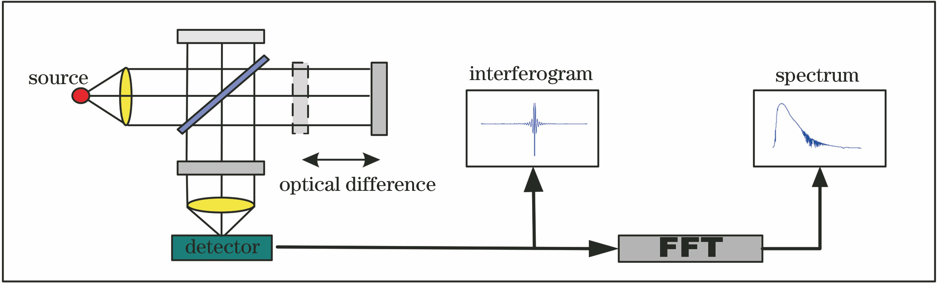
Fig. 1. FTIR system
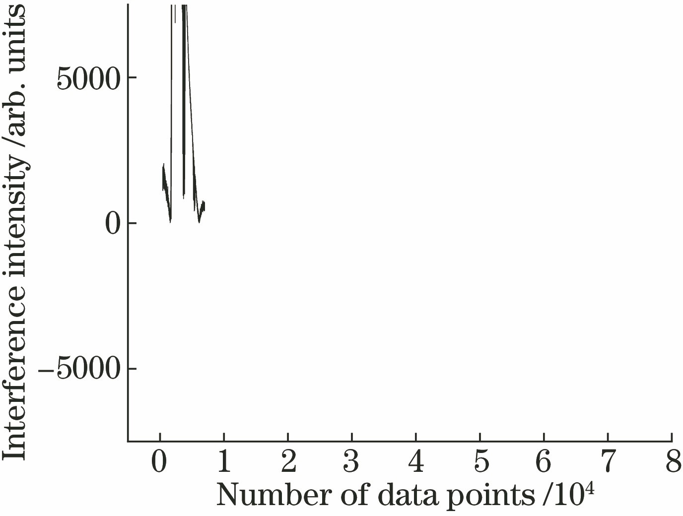
Fig. 2. Interferogram of CO
Fig. 3. Spectrum of CO
Fig. 4. Diagram of traditional data processing method
Fig. 5. Interferogram of ZPD position on left side of center of interference signal
Fig. 6. Interferogram of ZPD position on right side of center of interference signal
Fig. 7. Results of different data processing methods for the same group of interference signals with turbulent noise
Fig. 8. Comparison of spectra in 2100--2200 cm-1 band
Fig. 9. Amplitude of frequency response of Hanning windows
Fig. 10. Flowchart of new data processing method
Fig. 11. Experimental system
Fig. 12. Spectrum of CO with concentration of 1%
Fig. 13. Spectrum of CO with concentration of 1% in 2240--2050 cm-1 absorption band
Fig. 14. Spectrum of CO with concentration of 1% (with turbulent noise)
Fig. 15. Spectrum of CO in 2240--2050 cm-1 absorption band
Fig. 16. Spectrum of interference signal obtained by new data processing method
Fig. 17. Spectrum of CO in 2240--2050 cm-1 absorption band obtained by new method
Fig. 18. Spectrum of interference signal obtained by traditional data processing method
Fig. 19. Spectrum of CO in 2240-2050 cm-1 absorption band obtained by traditional method
Fig. 20. Nonlinear fitting of 1% CO absorption line
|
Table 1. SNR of results obtained by two methods
|
Table 2. Commonly used spectral window coefficient
| ||||||||||||||||||||||||||||||||||
Table 3. Results of concentration and correlation of two methods
|
Table 4. Concentration and correlation obtained by new method

Set citation alerts for the article
Please enter your email address
© Copyright 2018-2021 | Chinese Laser Press. All Rights Reserved 沪ICP备15018463号-20