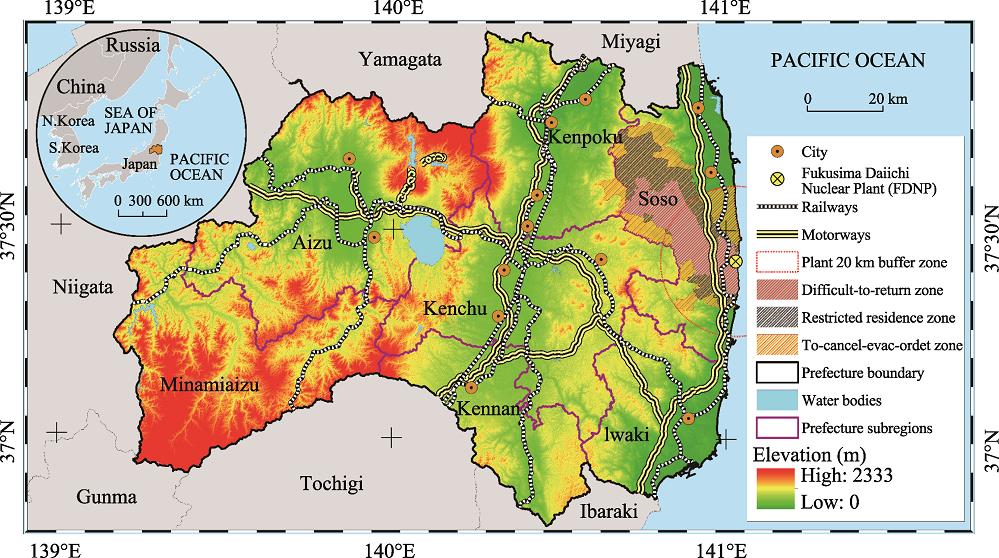
Fig. 1. Fukushima prefecture and its administrative boundaries, topographic features, transportation lines, and evacuation zones after the Fukushima Daiichi Nuclear Plant disaster (as of September 2015)
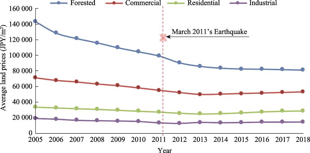
Fig. 2. Changes in land prices averaged by land type in Fukushima prefecture (2005-2018)
Fig. 3. Methodological framework of the study
Fig. 4. The distribution of land price samples in the study area
Fig. 5. Fitted semi-variograms for the kriging models for the year 2015: (a) Exp: Exponential (b) Gau: Gaussian (c) Sph: Spherical. The nugget, range, and sill values and the mathematical models are shown in the bottom right corner
Fig. 6. The results of the regression kriging for the year 2015 using the exponential model (upper), Gaussian model (middle), and spherical model (lower). On the left are the estimated log-transformed land prices using regression kriging. On the right are the validation errors in the training samples. Capital letters denote major cities within Fukushima prefecture, which are A: Fukushima, B: Koriyama, C: Iwaki, D: Aizuwakamtsu, and E: Shirakawa
Fig. 7. Land price maps for the year 2015 predicted from officially published land price observations using regression kriging based on three mathematical models (ordered from left to right): (1) Krig.EXP: Exponential model, (2) Krig.GAU: Gaussian model, and (3) Krig.SPH: Spherical model
Fig. 8. Boxplots of performance of machine learning methods in terms of the MAE, the RMSE, and R2 for the year 2015
Fig. 9. Observed land prices vs. predicted land prices for the year 2015 in the testing samples by different machine learning methods (ordered from left to right, up to down): (1) GLM: generalized linear model, (2) GAMS: generalized linear model using splines, (3) SVMLinear: support vector machines with linear kernel, (4) MARS: multivariate adaptive regression spline, (5) kNN: k-nearest neighbors, (6) SVMRadial: support vector machines with radial basis function kernel, (7) Cubist, (8) GBM: stochastic gradient boosting and (9) RF: random forest
Fig. 10. Land price maps for the year 2015 predicted from officially published land price observations using machine learning algorithms (ordered from left to right, up to down): (1) GLM: generalized linear model, (2) GAMS: generalized linear model using splines, (3) SVMLinear: support vector machines with linear kernel, (4) MARS: multivariate adaptive regression spline, (5) kNN: k-nearest neighbors, (6) SVMRadial: support vector machines with radial basis function kernel, (7) Cubist, (8) GBM: stochastic gradient boosting and (9) RF: random forest
Fig. 11. Maps of differences in the 2015 land prices between the best-performing machine learning algorithms: (1) RF: Random Forest, (2) Cubist, (3) MARS: Multivariate Adaptive Regression Spline and (4) GAMS: Generalized Linear Model using Splines and kriging exponential model. A1, A2, A3, and A4 show zoomed-in maps of Koriyama city and its outskirts
Fig. 12. Area percentage of RF- and krig.EXP-based estimated land price for the year 2015 distributed by predefined ranges in Fukushima prefecture and its subregions
| Estimation approach | Study | Study area | Method(s) | Mapping | Objective | Highlighted results |
|---|
| Hedonic models | (Löchl, 2006) | Canton Zurich, Switzerland | Hedonic regression | Yes | Developing an estimation model of rent and land prices | Two classified maps of land prices for residential and commercial uses | | (Kim and Kim, 2016) | Seoul, South Korea | OLS and spatial regression models | No | Estimation of land value using OLS and generalized regression models | Spatial error model (SEM) found to be the best of the tested models | | (Hilal et al., 2016) | Côte-d’Or, France | OLS | No | Estimation of the price of agricultural lands at cadastral levels based on previous real estate transactions | Hedonic prices were calculated based on a range of attributes influencing agricultural lands most notable time effects | | Geostatistical methods | (Luo and Wei, 2004) | Milwaukee, Wisconsin, USA | Kriging | No | Predicting urban land values of different land use categories using kriging models | Overall average standard error of 2% | | (Chica-Olmo, 2007) | City of Granada, Spain | Kriging and cokriging | Yes | Estimating and mapping housing prices using kriging and cokriging approaches | Cokriging has a lower standard error compared with that of kriging | | (Inoue et al., 2007) | Tokyo 23 wards, Japan | Kriging | Yes | Mapping estimated land prices in Tokyo’s 23 wards from 1975 to 2004 | Kriging model-based results were more accurate than those for OLS with the average error ranging from 2% to 10% | | Geostatistical methods | (Tsutsumi et al., 2011) | Tokyo metropolitan area, Japan | Regression kriging | Yes | Developing a system to estimate and map residential land price in the Tokyo metropolitan area | 10% was the average error ratio for the exponential model but 18.3% for the Gaussian model | | (Kuntz and Helbich, 2014) | Metropolitan area of Vienna, Austria | Kriging and cokriging | Yes | Mapping predicted real estate prices | Universal cokriging showed better results in terms of cross-validation results | | (Chica-Olmo et al., 2019) | City of Grenada, Spain | Regression and universal cokriging | Yes | Spatiotemporally estimating housing price variations 1988-2005 | Regression cokriging was found to be slightly better | | (Palma et al., 2019) | Italy | Jackknife kriging | No | Predicting real estate prices based on socioeconomic factors for the period 2014-2016 | Accuracy of the model improved when considering the spatio-temporal correlation | | Machine learning algorithms | (Gu et al., 2011) | A district of Tangshan city, China | Hybrid genetic algorithm and support vector machine model (G-SVM), Grey Model (GM) | No | Forecasting housing prices | G-SVM outperformed GM in many aspects | | (Antipov and Pokryshevskaya, 2012) | Saint Petersburg, Russia | Machine learning algorithms | No | Estimating residential apartments | Random forest was found to be the most robust among all methods | | (Wang et al., 2014) | Chongqing city, China | SVM optimized by particle swarm optimization (PSO), BP neural network | No | Forecasting real estate price based on PSO-optimized SVM compared to other BP neural network | PSO-SVM showed higher forecasting accuracy than BP neural network | | (Park and Bae, 2015) | Fairfax County, Virginia, USA | Machine learning algorithms (C4.5, RIPPER, Naïve Bayesian, and AdaBoost) | No | Prediction of housing prices using different machine learning methods | RIPPER model outperformed all selected methods | | Comparison of various approaches | (Bourassa et al., 2010) | Jefferson County, Kentucky, USA | OLS, nearest neighbors, geostatistical and trend surface models | No | Comparing the outcomes of several methods estimating house prices | The geostatistical model showed better results in terms of prediction errors | | (Sampathkumar et al., 2015) | Chennai metropolitan area, India | Multiple regression and neural network | No | Modeling and estimation of land prices based on economic and social factors | Neural network and multiple regression performed well with a slight superiority of the former | | (Hu et al., 2016) | Wuhan city, China | Empirical Bayesian kriging (EBK), GWR, OLS | Yes | Modeling and visualizing dependency of urban residential land price and the influential variables | Estimated coefficients of variables impacting land prices depend on the location based on GWR results which outperformed OLS | | (Schernthanner et al., 2016) | Potsdam, Germany | Hedonic regression, kriging, and random forest | Yes | Comparing estimated rental prices by three methods and visualize the outcome | RF found to be the most accurate method |
|
Table 1. Descriptive list of reviewed literature regarding land price estimation/mapping grouped by estimation approach: (1) hedonic models, (2) geostatistical methods, (3) machine learning algorithms, and (4) comparison of various approaches
| Category | Model | Abbreviation | R package |
|---|
| Geostatistical | Universal kriging | Exponential | krig.EXP | gstat (Pebesma, 2004) | | Gaussian | krig.GAU | | Spherical | krig.SPH |
|
Table 2. The three mathematical models used for kriging and their abbreviations
| Category | Model | Abbreviation | R package |
|---|
| Linear | Generalized linear model | GLM | base | | Generalized additive model using splines | GAMS | mgcv | | Support vector machines with linear kernel | SVMLinear | kernlab | | Nonlinear | Multivariate adaptive regression spline | MARS | earth | | k-nearest neighbors | kNN | base | | Support vector machines with radial basis function kernel | SVMRadial | kernlab | | Regression trees | Cubist | Cubist | Cubist | | Stochastic gradient boosting | GBM | gbm (Ridgeway, 2005) | | Random forest | RF | randomForest (Breiman, 2001) |
|
Table 3. Summary of spatial prediction models used in this study: Linear, nonlinear, and regression trees models are grouped as proposed by Kuhn and Johnson (2013). Abbreviations are used to refer to each method in the manuscript
| Explanatory variables | Data | GIS function | Variable description | Abbreviation |
|---|
| Distance to the nearest railway station (m) | Railway stations | Near | Calculated using the railway stations layer | Distance | | Area of rice fields [m2] | Land uses within a square kilometer | Spatial Join | The areas of different land-uses within one square kilometer classified according to the National Land Numerical Information | Paddy | | Area of other agricultural land (m2) | Agricultural | | Area of forests (m2) | Forests | | Area of uncultivated land (m2) | Uncultivated | | Area of roads (m2) | Roads | | Area of railways (m2) | Railways | | Area of other land uses (m2) | Other uses | | Area of water bodies (m2) | Water | | Area of seashore (m2) | Seashore | | Area of the surface of the sea (m2) | Sea | | Area of golf courses (m2) | Golf | | Dummy variable for urbanization promoting area | Promoted urbanization areas | Spatial Join | A dummy variable; if the point location falls inside the area, the variable value receives 1, else 0 | Promotion | | Population density (persons/km2) | Population | Spatial Join | Calculated using the population data of 2015 for every minor municipal district | Density | | Number of enterprises | Enterprises | Spatial Join | Statistical GIS data of 2015 for every minor municipal district | Enterprises | | Number of employees | Employees | Employees | | Elevation (m) | DEM | Extract Multi Values to Points | Elevation of the point location | Elevation |
|
Table 4. List of explanatory variables selected in this study with their data sources and the related abbreviations
| Data layers | Source | Year |
|---|
| Land price observations (published and prefectural) | National Land Numerical Information | 2015 | | Railway stations | 2015 | | Land uses within 1 km2 area and their areas | 2014 | | Promoted urbanization areas | 2011 | | Population of every minor municipal district | Statistics Bureau of Japan | 2015 | | Number of enterprises and employees of every minor municipal district | | DEM | USGS | - |
|
Table 5. Overview of datasets used in the study, their sources, and the year of release
| Variables | Unit | Coefficients’ estimate |
|---|
| Intercept | - | 4.439 | *** | | Distance to the nearest railway station | m | -2.09 × 10⁻⁵ | *** | | Population density | persons/km2 | 3.104 × 10⁻⁵ | *** | | Area of rice fields | m2 | -3.935 × 10⁻⁷ | *** | | Area of other agricultural land | m2 | -4.731 × 10⁻⁷ | *** | | Area of forests | m2 | -2.733 × 10⁻⁷ | *** | | Area of uncultivated land | m2 | -7.437 × 10⁻⁷ | . | | Area of roads | m2 | 7.211 × 10⁻⁷ | ** | | Area of railways | m2 | -3.301 × 10⁻⁸ | | | Area of other land uses | m2 | -8.97 × 10⁻⁸ | | | Area of water bodies | m2 | -3.086 × 10⁻⁷ | *** | | Area of seashore | m2 | -1.922 × 10⁻⁶ | | | Area of the surface of the sea | m2 | -1.25 × 10⁻⁷ | | | Area of golf courses | m2 | -5.843 × 10⁻⁸ | | | Dummy variable for urbanization promoting area | - | 1.819 × 10⁻¹ | *** | | Elevation | m | -1.556 × 10⁻⁴ | ** | | Number of enterprises | - | 3.363 × 10⁻⁴ | ** | | Number of employees | - | -2.951 × 10⁻⁵ | * | | Number of samples = 1092; residual standard error = 0.1683, multiple R2 = 0.7408, adjusted R2 = 0.7349; F-statistic = 125.7, p-value = < 2.2 × 10⁻¹⁶*** = sign. at 1% level ** = sign. at 5% level |
|
Table 6. Regression results with detailed explanatory variables and their estimated coefficients
| Mathematical models | Validation | Cross-validation |
|---|
| RMSEV (%) | RMSECV (%) |
|---|
| Exponential | 15.32 | 15.1 | | Gaussian | 15.86 | 15.57 | | Spherical | 15.57 | 15.5 |
|
Table 7. Prediction errors of validation and cross-validation tests for the three kriging models
| Method | 10-fold cross-validation | Testing samples | Difference |
|---|
| MAE (%) | RMSE (%) | R2CV (%) | R2test (%) | R2CV (%) - R2test (%) |
|---|
| Linear | GLM | 13.50 | 17.29 | 72.47 | 59.94 | +12.53 | | GAMS | 12.03 | 15.37 | 78.13 | 68.72 | +9.41 | | SVMLinear | 13.38 | 17.25 | 72.73 | 59.12 | +13.61 | | Nonlinear | MARS | 12.11 | 15.52 | 77.90 | 70.78 | +7.12 | | kNN | 13.38 | 17.35 | 72.24 | 68.03 | +4.21 | | SVMRadial | 12.55 | 16.27 | 75.53 | 70.02 | +5.51 | | Regression tree | Cubist | 12.19 | 15.60 | 77.72 | 72.74 | +4.98 | | GBM | 12.16 | 15.68 | 77.40 | 70.83 | +6.57 | | RF | 11.39 | 14.97 | 79.17 | 77.68 | +1.49 |
|
Table 8. Prediction errors and accuracy of machine learning methods