Maps depicting the spatial distribution of land prices are an essential reference in urban and regional planning during post-disaster recovery periods and beyond. Such maps are employed as one of the strategic assets for various purposes, such as optimally allocating land resources (Hu et al., 2016), developing special land policies for potential investors, and making economically justified planning decisions either by planning authorities or ordinary citizens (Cellmer et al., 2014). It is always critical for key investors and planners to investigate the economic value of land before starting any prospective project at the local and regional levels. However, it is more challenging to examine the variation in land prices in a wide area. This is due to the incredible budget- and time-consuming process behind extracting land price maps covering a whole region, which necessitates costly and lengthy field surveys. Furthermore, the available samples do not usually cover the entire study area in question as the data is collected from dispersed locations. For this reason, a specific spatial analysis is required to estimate land values at any given site.

Geographic Information Systems (GIS) coupled with spatial statistics provide the necessary tools for estimating land prices and extracting accurate maps based on rigorous mathematical models. In recent years, several studies with the objective of estimating and/or mapping land prices have been carried out. However, they differ significantly when it comes to the methodologies followed, the explanatory variables considered, and the spatial scale of the study area selected. Table 1 lists reviewed studies related to the prediction and/or mapping of land and housing prices worldwide, grouped by the implemented estimation approaches that can be split into four categories: (1) hedonic models, (2) geostatistical methods, (3) machine learning algorithms, and (4) hybrid models or multiple approaches compared. Although the relationship between housing prices and land prices has been a controversial topic in terms of the relevant determining factors considered and the statistical models applied (Wen and Goodman, 2013), we present studies that dealt with both.

Hedonic modeling is based on the fact that a land parcel or a house is a function of its characteristics (Caplin et al., 2008) and is mostly expressed by a linear regression equation of structural, socioeconomic, and environmental factors. This modeling can be implemented using ordinary least squares (OLS; Crespo and Grêt-Regamey, 2013). It was among the first techniques for evaluating and predicting land or house prices and has long been used by many researchers, including Löchl (2006), Kim and Kim (2016), Bourassa et al. (2010), Schernthanner et al. (2016), and Hilal et al. (2016), among others. These models generally have several limitations because they depend on the availability of a large dataset which has high costs and requires time-consuming field surveys (Kuntz and Helbich, 2014). Following the development of regression modeling techniques, and taking into account the spatial nature of land price observations, other methods have been developed based on spatial autocorrelation and spatial heterogeneity (Crespo and Grêt-Regamey, 2013). Geographically weighted regression (GWR; Brunsdon et al., 1998) is an example of a regression-based method that incorporates the spatial dimension of attributes within the analysis, and many studies showed good results compared to traditional hedonic models. However, when the prediction accuracy of GWR is compared with those of geostatistical methods, many studies have reported low accuracy for GWR compared to that of kriging, for instance (e.g., Kuntz and Helbich, 2014). Kriging and cokriging models have been implemented for different topics in geosciences (e.g., remote sensing, climatology, and agriculture) and have shown robust performance in terms of estimation errors. Due to their flexibility, Palma et al. (2019) affirmed the capability of geostatistical methods to tackle socioeconomic phenomena as well, which can be seen in the number of studies conducted to model land or house rental prices (e.g., Chica-Olmo, 2007; Chica-Olmo et al., 2019; Kuntz and Helbich, 2014; Luo and Wei, 2004; Tsutsumi et al., 2011). Most recently, new studies introduced machine learning (ML) algorithms as possible alternatives to hedonic models and geostatistical methods to describe spatially and temporally the distribution of land prices. Gu et al. (2011), for instance, developed a hybrid model of a genetic algorithm and the random forest (RF) algorithm to forecast housing prices in a Chinese district of Tangshan city. Antipov and Pokryshevskaya (2012) conducted a comparative study of 10 ML methods to estimate residential apartments in St. Petersburg. A similar study was carried out by Park and Bae (2015) to model housing prices in Fairfax County (in the United States) by comparing various ML algorithms. Other efforts have been made to empirically compare the performance of two or more approaches among different ML, hedonic, and geostatistical techniques. For example, Bourassa et al. (2010) compared the house prices estimation results of OLS, a two-stage nearest neighbors’ residual procedure, geostatistical methods, and trend surface models based on around 13,000 transactions from Louisville, Kentucky. According to the authors, the geostatistical approach based on the robust exponential mathematical model performed best. In a similar vein, Sampathkumar et al. (2015) investigated land price trends by employing multiple regression and neural networks to model land prices in the Indian Metropolitan Area of Chennai. They found that both approaches performed well; the second method was slightly better. Schernthanner et al. (2016) used hedonic regression, kriging, and the random forest algorithm to map the estimated rental prices in the German city of Potsdam. The authors concluded that the RF algorithm is the most accurate method for forecasting and mapping land prices in the region.

Overall, comparative spatial studies on estimation of land prices across a macro-area implementing geostatistical methods and ML algorithms are scarce. Moreover, most of the papers used different datasets for each approach, which may lead to data-dependent results. Additionally, most studies did not map the spatial distribution of price estimation and consequently, missed helpful, informative statistics in a given study area. The present study may contribute considerably to the increasing academic works on land prices by filling these research gaps, as it aims at empirically comparing the outcome of three mathematical models of regression kriging and nine of the most frequently used ML algorithms. Specifically, this paper addresses the following objectives: (1) mapping the estimated land prices using regression kriging and empirically assessing the outcomes, (2) mapping the predicted land prices using nine different ML algorithms and empirically evaluating the results, and (3) qualitatively and quantitatively comparing the results of the two approaches.

The remainder of this paper is structured as follows. In Section 2, light is shed on land price estimation and mapping in Japan. In Section ‎3, the study area and the spatial estimation techniques used are introduced, an overview of the data sources and the explanatory variables considered is provided, the methodological framework is presented. In Section ‎4, the results of the different analyses are provided and compared. In Section ‎5, the results and limitations of the study are discussed, and the conclusions are presented.

In Japan, land is a precious natural resource, as the archipelagic country has limited flat areas and has been experiencing fast urban expansion for decades. Several factors influence the land price, including population density, proximity to economic hotspots (e.g., central business district (CBD)), accessibility to means of transportation and geophysical characteristics (e.g., location, topography, and land use). In general, most of these factors are related to urban growth. Capozza and Helsley (1989), among others (e.g., Arnott and Lewis, 1979; Capozza et al., 1986), confirmed that there is a positive proportional relationship between the speed of urban growth and land prices.

Moreover, as one of the most natural disaster-prone countries in the world, Japan is continuously involved in post-disaster reconstruction and redevelopment plans in affected regions. These plans necessitate developing special land policies based on economically justified decisions supported by accurate references, such as land price maps assessing existing assets to encourage potential infrastructure investments, for instance. Therefore, land price is an important key for allocating land resources for wise regional and urban planning and development, specifically in big cities and metropolitan areas characterized by recurrent changes in population and infrastructures (Hu et al., 2016). For these reasons, monitoring land prices has become a priority issue for decision-makers and under intensive investigation and analysis by academic researchers. In the Japanese context, spatial data for land prices is published every year by local and prefectural governments. Although this data may be downloaded free of charge from the internet, it is available only as GIS vector points and in a limited number of samples, which does not provide complete information for all market participants (Inoue et al., 2007). Because of this limitation, developing an approach for accurately estimating and mapping land prices in all locations across a given study area based on rigorous statistical principles is needed. Many estimation methods have been used separately, including geostatistics-based models and machine learning algorithms. However, comparative analyses that investigate the methods with precise results are relatively scarce.

There have been many empirical studies with the aim of estimating land prices in Japan, focusing mainly on the Tokyo Metropolitan Area (TMA). For instance, Shimizu and Nishimura (2007) employed a hedonic approach based on OLS to develop commercial and residential land price indices for the core wards of the TMA, and then to investigate the structural changes in land pricing between 1975 and 1999 reflecting the pre-bubble, bubble, and post-bubble periods. The authors found differences in price structure due to location and fluctuations between supplier pricing and end-user preferences. Using the same estimation approach, Sasaki and Yamamoto (2018) estimated hedonic residential prices in the TMA by introducing “regional vulnerability” and “accessibility to destination stations” as two new explanatory variables. To the extent of our knowledge, however, only two English-language papers with the aim of mapping estimated land prices using GIS were published. The first study was conducted by Inoue et al. (2007) in which the authors used universal kriging to estimate land prices in Tokyo’s 23 wards spatially and temporally over 30 years (from 1975 to 2004). By comparing kriging results with those of the OLS model, the authors found that the former performed better, with an estimation error ranging from 2% to 10% except during the period from 1986 to 1991 (approximately 20%) when the Japanese economy experienced harsh stagnation due to the fall in land prices and the stock price bubble (Shimizu et al., 2015). The second study was carried out by Tsutsumi et al. (2011) in which they developed a computer-aided system that combines GIS and statistical theories to extract land price maps of the TMA based on free officially published residential land price observations. Regression kriging was used in the study, where two mathematical models of semi-variograms (exponential and Gaussian) were employed. The results showed that the exponential model performed better with a 10% average error ratio; the ratio was 18.3% for the Gaussian model. This study was a useful reference for the present paper, mainly in terms of the selection of explanatory variables and the regression kriging analysis.

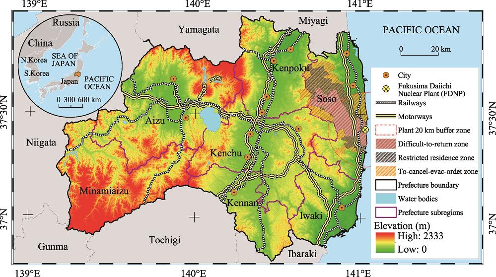
The study area is Fukushima prefecture (Figure 1) located in the Tohoku region, Japan. The prefecture is divided into seven subregions (Aizu, Iwaki, Minamiaizu, Kenchu, Kennan, Kenpoku, and Soso). According to the Ministry of Internal Affairs and Communications, approximately 1,914,000 residents live in an area of 13,784 km² with a total population density of 140 residents per square kilometer (MIAC, 2016). The region is characterized by a mountainous landscape mainly in the western region predominantly in Minamiaizu with the elevation ranging between 0 and 2333 m above sea level. Major cities, which are well connected by railways and highways, are located in flat areas primarily in the coastal areas of Iwaki and Soso; the central region located in Kenpoku, Kenchu, and Kennan; and in the northeast region of the prefecture specifically in the Aizu subregion. Following the 2011 Fukushima Daiichi accident, the prefectural government designated nuclear-contaminated areas as evacuation zones (Figure 1). These areas, located mainly in Soso and Kenpoku, are divided into three zones according to radiation levels and authorized entry, business operations, and resident levels. Generally, previous residents are prohibited from living in all zones with some exceptions in areas labeled as “restricted residence zone” and “evacuation-order cancellation preparation zone.” However, business operations are fully permitted in the outer zone, but are partially granted in the restricted-residence zone.

Since the disastrous accident at the Fukushima Daiichi Nuclear Plant in the aftermath of the Great Earthquake of 2011, public opposition to nuclear power has intensified in Japan generally, and in Fukushima prefecture in particular given that it was the most affected prefecture (Tsujikawa et al., 2016). This fact forced the prefectural government to rely more on clean energy resources to improve energy security (Wang et al., 2016), as part of a promising vision to become renewable energy self-sufficient by 2040 (Derdouri and Murayama, 2018).

Consequently, the prefectural government and interested investors are looking for optimal locations in the prefecture to develop renewable energy projects (e.g., solar, wind, and hydro). However, for this site suitability exercise to be achieved, various evaluation criteria including “land price” are required. For instance, in a study carried out by Tegou et al. (2010) in which they evaluated the suitability of wind power plants on the Greek island of Lesvos, the authors considered the criterion “land value” to estimate the economic value of the area, among other factors. Likewise, Derdouri and Murayama (2018) extracted the map of the ideal sites for installing new wind parks in Fukushima prefecture. The authors, through a survey among local wind experts and different stakeholders, concluded that the evaluation factor “land price” is among the five most important criteria in the suitability analysis of wind farms in the prefecture. Therefore, the prefecture of Fukushima was selected as the study area of the present study.

The prefecture has been the center of national and even global attention since 2011. Multiple studies on the effects of the 2011 nuclear disaster on land prices were carried out. Yamane et al. (2013), Tanaka and Managi (2016), and Kawaguchi and Yukutake (2017) concluded that soil contamination resulted from the accident caused land prices to fall. However, these studies analyzed only short-term impacts. In contrast, Nishimura and Oikawa (2017) examined the long-term effects of the accident on land prices in the prefecture and areas surrounding nuclear reactors in Japan and found that the impacts are not significant. This is shown in Figure 2 illustrating the average values of land prices by land category from 2005 to 2018 in the prefecture based on local and prefectural governments’ observation surveys. Before 2011, commercial, residential, and industrial land parcels had experienced continuous slight decreases in value since 2005 by around 16,230 JPY/m², 6340 JPY/m², and 5492 JPY/m², respectively. However, forest land, which represents the most valuable type of land in the prefecture, with an average price of 143,200 JPY/m² in 2005, lost approximately 44,067 JPY/m² of its value from 2005 to 2011. The cost of these types of land dropped sharply after the 2011 earthquake, losing another 8839 JPY/m² by 2012. In contrast, minor drops in values were observed for the other types of land post-earthquake. Starting in 2013, we can see the prices for all types are generally steady with an observed slight decrease in the value of forest land compared to a small increase in the value of commercial, residential, and industrial land. Overall, from a historical perspective, the 2011 Fukushima Daiichi accident caused land prices to drop for a short period until 2013. Then these values stabilized with slight changes during the following years.

The interpolation methods proposed in this research are divided into two groups: geostatistical and machine learning based. The former refers to kriging, which is a widely applied method for interpolation developed by South African statistician Danie G. Krige (Krige, 1951) in the early 1950s. It deals with spatial correlations to compute the best linear unbiased predictor values at any unobserved location by relying on observed values of explanatory variables. The latter is a collection of algorithms that train machines to detect possible correlations in observations’ data. Tables 2 and 3 summarize the spatial estimation methods used in this study in addition to the R packages used for every model. The R geostat package (Pebesma, 2004) was used to perform kriging, whereas the caret package (Kuhn, 2008) was employed to implement machine learning methods. More details about these techniques are found in the following sections.

3.2.1 Regression kriging

The first spatial estimation technique is regression kriging (Hengl, 2009; Hengl et al., 2007). The idea of multiple linear regression is to find the best linear equation that describes the relationship between two or more explanatory variables and the response variable. In this case, these variables are in the form of geographic data, and the following linear model is used to estimate the land price at any location:

where s refers to each location, and y_s is the value of the response variable, which in this case is the land price value at location s. Due to the skewed distribution of the land price values, we decided to work with the log10-transformed values instead. In addition, i denotes the index of the explanatory variables; its values are within the range (1, 2 … N) where N is the total number of explanatory variables considered. β₀ and β_i are the parameters of the regression line. x_i,s represents the values of the explanatory variables at location s. ε_s is the residuals of the regression model.

Kriging employs semi-variograms which are functions measuring the strength of the spatial correlation as a function of distance based on Tobler’s first law of geography that everything is related to everything else, but near things are more related than distant things (Tobler, 1970). The semi-variogram is described in the following equation:

where N is the number of pairs of sample points separated by distance h, z(s_i) is the value of the target variable at some sampled location, and z(s_i+h) is the value of the neighbor at distance s_i+h.

The three mathematical models, namely, exponential, Gaussian, and spherical, represented by equations (3), (4), and (5), respectively, are used to fit the semi-variogram to the curve to the empirical data of land prices. Consequently, the important characteristics (i.e., sill, range, and nugget) are determined for each model:

To evaluate the performance of the models, validation and cross-validation are applied using root mean squared error (RMSE), which is a widely used formula to measure the error rate of a regression model. The following equation represents the RMSE:

where $\hat{y_{i}}$ and y_i represent the predicted and real values, respectively, and n is the total number of validation points.

3.2.2 Machine learning

Machine learning is a collection of mathematics-, computation- and statistics-based methods that aim to automatically learn rules and dependencies from examples and data (Ratle et al., 2010). In this study, we considered the nine machine learning algorithms listed in Table 3. These models can be classified into three categories following Kuhn and Johnson’s (2013) proposition: (1) linear, (2) nonlinear, and (3) regression trees.

The three models of the first category are the generalized linear model (GLM), generalized additive model using splines (GAMS), and support vector machines with linear kernel (SVMLinear). They are practical in linear relationships between the dependent variable and covariates, and they seek to find estimated coefficients that minimize the sum of the squared errors. These models can be interpreted easily by analyzing the estimated coefficients. Moreover, due to the ability to compute standard errors, the significance of every covariate can be deduced. However, from a real-world perspective, they oversimplify complex problems especially in the case of limited covariates.

Nonlinear models include multivariate adaptive regression spline (MARS), k-nearest neighbors (kNN), and support vector machines with radial basis function kernel (SVMRadial). In contrast to linear models, these models do not require knowing the form of the relationship between the dependent variable and explanatory variables beforehand.

The third category comprises tree-based models, including Cubist (Cubist), stochastic gradient boosting (GBM), and random forest (RF). They are considered nonlinear models as well; however, they were categorized in a separate group due to their wide popularity. These models split the data into partitions based on one or more nested conditional statements [If … Then] according to the predictor values. Subsequently, for each partition, the outcome is determined.

Land value can be affected by various variables. According to Wen et al. (2018), these variables are frequently grouped into three types: (1) individual factors referring to the characteristics of the land parcel such as size and shape; (2) neighborhood factors related to the characteristics of the land parcel including socioeconomic variables, external environment, and amenities; and (3) location determinants depicting traffic patterns and distance to the CBD. In the literature, multiple authors have associated the economic value of land with variables such as population density, proximity to railways, schools, and other facilities. For example, Zhuang and Zhao (2014) analyzed the effects of land use and railway stations on land prices in Fukuoka city of Japan concluding that land prices near railway stations and commercial or industrial hotspots are usually high. The closer the land to these locations, the expensive it becomes. Likewise, Kanasugi and Ushijima (2018) examined the impacts of a scheduled-to-open high-speed railway on residential land prices. The authors reported an increase in land prices in the areas that shortened travel time to the TMA. Kok et al. (2014) examined the determinants of land prices in the metropolitan area of the San Fransisco Bay Area. Results indicated that elevation and job density among other geographic, topographic, and demographic factors, are strongly associated with land economic values. Tsutsumi et al. (2011) linked land prices in the TMA with population density and land use, among other factors. Adegoke (2014) investigated the factors determining the value of residential properties in the Ibadan metropolis in Nigeria. Adegoke found a significant relationship between land price and mainly the population density and level of development. Other studies have linked proximity to urban facilities, such as schools, parks, and sports-related venues with mainly residential prices in Singapore (Murakami, 2018), China (Liu et al., 2007), Kuwait (Mostafa, 2018), Spain (Chica-Olmo et al., 2019), and the United States (Clapp et al., 2008; Espey and Owusu-Edusei, 2001; Kiel and Zabel, 2008). In conclusion, the selection process of suitable factors depends mainly on various elements, such as the setting of the designated target area, type of land price (e.g., residential and commercial), and the availability of aspatial or spatial data.

In this study, we based the selection of explanatory variables on the literature by considering the following elements: (1) the land parcels are within urban and rural areas, (2) the land parcels are not only for residence purposes, and (3) the availability of free spatial data satisfying two necessary conditions in accordance with the following (Tsutsumi et al., 2011). First, the corresponding spatial data of each explanatory variable should cover the whole prefecture of Fukushima, so that the estimated land price can be calculated at any location within the study area. Second, the data should have been collected during the same year as much as possible (i.e., 2015). Table 4 shows the final list of the explanatory variables, where the column heading “Data” indicates the sources of data listed in Table 1, and “GIS function” refers to the ArcMap’s function that was used to extract the variable values from the data.

The present study exploits publicly available and no-cost data from different sources. Data on published and prefectural land price observations of the year 2015 was downloaded from the National Land Numerical Information download service¹ ( National Land Numerical Information download service. URL: http://nlftp.mlit.go.jp/ksj-e/gml/gml_datalist.html (in English))(Ministry of Land, Infrastructure, Transport, and Tourism) as GIS vector data. Other data layers were obtained from the same source, including railway stations, promoted urbanization areas, and a grid of 1 km2 cells containing information about the area of every land use. Data on population of 2015 census, number of enterprises, and employees of every minor municipal district was collected from the Statistics Bureau of Japan²(²Statistical GIS - Portal site for Japanese Government Statistics. URL: https://www.e-stat.go.jp/gis (in Japanese)). Finally, a digital elevation model (DEM) was downloaded using EarthExplorer of USGS³ ( ³United States Geological Survey. URL: https://earthexplorer.usgs.gov/). Table 5 summarizes the data used in this analysis and describes the sources of the data and the year of release.

The proposed methodology for this analysis is illustrated in Figure 3. It consists of three parts: (1) data preparation using GIS software ArcGIS, (2) geostatistical analysis employing the software RStudio (https://www.rstudio.com/), and (3) machine learning modeling using RStudio. A detailed explanation of every part is given in the following sections.

Data preparation: The first part consists of preparing a points-data layer A and points grid B. The former contains the merged observations of land prices (resulted from published and prefectural observation surveys) covering the extent of the study area, including the six neighboring prefectures: Miyagi, Yamagata, Niigata, Gunma, Tochigi, and Ibaraki. The extent of the study area was considered in this analysis to include more observation points and to make them distributed all over Fukushima prefecture as shown in Figure 4. The latter is the layer of the central points of a 1 km² cell mesh where the horizontal distance between every two points is about 1100 m, and the vertical distance is approximately 900 m. Layer A and grid B contain the same fields representing the explanatory variables, including the distance to the nearest railway station, population density, elevation, surface of every land use within an area of 1 km², and a field representing whether a point falls within the promoted urbanization zone or not. For every point of A and B, the values of these explanatory variables are extracted using the Near, Spatial Join, and Extract Multi Values to Points functions in ArcMap.

Geostatistical analysis: This part includes a two-step procedure which is regression kriging. Based on Matheron’s theory, a regionalized variable can be modeled as a sum of two components: deterministic and stochastic (Szymanowski et al., 2013). First, multiple regression analysis is applied with the assumption that the dependent variable (log-transformed land prices) is spatially correlated with a collection of explanatory variables in which their values are known at every location in the study area. Second, as explained in Section ‎3.2.1, we use three mathematical models (exponential, Gaussian, and spherical) to fit the variogram. Consequently, we use the fitted semi-variogram for every model to predict the values log-transformed land prices at all points of grid B. We then perform validation and cross-validation to assess the accuracy of the results of the three models by calculating the RMSE.

Machine learning modeling: The last part of the analysis consists of running machine learning methods using R’s caret library. By applying the ArcMap function Point to Raster on grid B, rasters representing explanatory variables are created. Thirteen machine learning algorithms are applied. We randomly split the observation samples into training samples (70%) and testing samples (30%). To compare the performance of these methods, the same training and testing samples were used for both approaches.

Before the geostatistical analysis and machine learning modeling were carried out, linear regression analysis was performed to find the relationship between selected explanatory variables and the independent variable (i.e., log-transformed land prices). Table 6 lists the regression parameters and their estimates calculated using the generalized least-square method. As expected, the coefficients of “population density,” “area of roads,” “area of railways,” and “dummy variable for urbanization promoting area” are positive. However, those for “distance to the nearest station” and “elevation” are negative, because the price of land decreases when the land is farther away from the nearest railway station or when the land is located in a mountainous area.

Regarding the accuracy of the regression model, the output F-statistic = 190.1 (p-value < 2.2 × 10^-16) indicates that we should reject the null hypothesis that the explanatory variables collectively do not affect land prices. The adjusted R² refers to the total percentage of sample points explained by the regression model. In this case, the total variation in the land price of about 73% of the points is explained by the explanatory variables.

For the geostatistical analysis, three mathematical models were used to perform kriging. Figure 5 illustrates the final corresponding fitted semi-variograms. All three models have nugget and sill values that are relatively equal to 0; however, the range of the krig.SPH model (1438 m) is approximately two times the krig.EXP’s (644 m) and the krig.GAU’s (760 m).

Figure 6 shows the results of the regression kriging using exponential, Gaussian, and spherical models, respectively. The maps on the left present the prediction results of log-transformed land prices, whereas the maps on the right show their validation errors. The validation error maps show that land price values were underestimated within urban areas (< 10 km) mainly in Fukushima, Koriyama, and Iwaki cities. However, the prices were overestimated outside the urban domain (> 10 km). These fluctuations may be attributed to many possible reasons: (1) the high density of observation points within urban areas and the low density elsewhere, (2) the broad study area, and (3) the use of a single model to predict prices within and outside urban areas.

The accuracy of the results of the kriging models was evaluated using validation and cross-validation approaches. Table 7 shows the RMSE values calculated using both methods. The models’ prediction errors are relatively equal, which range approximately between 15.1% and 15.9% for validation and cross-validation. The exponential model gives slightly better outcomes in both tests, which coincide with the result found by Tsutsumi et al. (2011) as well as Chica-Olmo et al. (2019). Figure 7 shows the land price maps for the year 2015 compiled based on officially published observational data.

The performance of the nine machine learning methods was assessed in terms of the mean absolute error (MAE), the RMSE and R². Additionally, testing samples were used to calculate the overall accuracy of the methods (Figure 8 and Table 8). The different performance indicators generally show good values for both validation tests. For 10-fold cross-validation, the MAE ranges from 11.39% to 13.50%, the RMSE from 15.37% to 17.35% and R² (R²_CV) from 72.24% to 79.17%. Using the testing samples, R² (R²_test) was calculated which has values ranging between 59.12% and 77.68%. The results indicate that these values are lower than R²_CV, and the difference ranges between 1.49% and 13.61%. Among these methods, RF seems to be the most robust method in terms of all performance indicators in agreement with the conclusions of Antipov and Pokryshevskaya (2012). Moreover, it can be found that regression tree algorithms generally score better results than nonlinear and linear methods as their RMSE values are above 70% in both validation tests.

Figure 9 presents the observed land prices and the predicted land prices for the year 2015 for the testing samples using different machine learning methods. Figure 10 presents the resulting maps of the predicted land prices of 2015 in the study area using machine learning algorithms. The spatial resolution of all maps is 100 m. All models show that land prices are spatially dependent on the distance to railways. The farther from railways the land, the higher the price. In remote areas around railways, the price ranges from 9500 JPY/m² to 12,000 JPY/m². Moreover, the most expensive land is located by all models within urban areas. Elevation was taken into consideration by most of the models except SVMRadial model that completely failed to consider topographic features, as it classified remote and mountainous areas in the southeastern (e.g., Mount Hiuchigatake with an elevation of 2356 m) and northern areas, for example, as high land price zones where the price exceeds 16,500 JPY/m². However, other models, including GAMS, MARS, kNN, and GBM, predicted medium (5000-9500 JPY/m²) land prices for the summit region.

For both analyses, we considered a similar set of training and testing samples to make the results of the different methods comparable. Consequently, we calculated the differences between the predicted land prices by the most robust machine learning methods (i.e., RF, Cubist, MARS, and GAMS) and the best-performing kriging based on the exponential model. The map results are illustrated in Figure 11. It can be seen that all maps have similar patterns across the study area, and the land price differences mostly range between -5000 JPY/m² and 5000 JPY/m².

In general, the kriging model estimates high values for land prices in areas around railways and urban areas, which can explain the negative difference values ranging from -5000 JPY/m² and -1000 JPY/m² in these areas. However, positive values indicating lower estimations of land prices by kriging compared to machine learning methods (except Cubist) are scattered across the study area and generally spotted in mountainous areas. In the same figure, A1, A2, A3, and A4 show zoomed-in maps of Koriyama city, which illustrate sharp fluctuations in differences in land prices within urban areas. Land prices estimated by kriging in the city center where there is dense population and near railway stations tend to be classified as very high (-149,570 JPY/m² to -20,000 JPY/m²) and high (-20,000 JPY/m² to -5000 JPY/m²) compared to other methods. The farther from the city center, the lower the land price differences.

In terms of the quantitative results of the two approaches, we compared the area percentages of land price ranges in the prefecture and its subregions. Given their superiority compared to the other models of each approach, RF and krig.EXP are considered. Areas of designated evacuation zones resulting from the Fukushima Daiichi accident were excluded in this analysis. For the sake of simplicity, we classify the degree of prices according to the following classification: (1) low price: [500-6000 JPY/m²], (2) medium price: [6001-10,000 JPY/m²], and (3) high price: [10,001-320,000 JPY/m²]. The results are illustrated in Figure 12. In general, similarities between percentage values of RF and krig.EXP can be seen in most subregions and for almost all price ranges except for low-price ranges [4001-6000 JPY/m²] and [6001-12,000 JPY/m²]. In the whole prefecture, both distribution graphs of the area percentage of land price based on RF and krig.EXP follow a normal distribution. It can be seen that more than 80% of the land of the prefecture cost between 4000 JPY/m² and 12,000 JPY/m². Minamiaizu is the cheapest subregion in terms of the economic value of land, with approximately 95% of the land costing less than 10,000 JPY/m². This can be attributed to the vast area of remote and mountainous areas, and likely the lack of an economic hotspot in the region. Neighboring subregions Aizu, Kennan, and Kenchu are not as cheap with 94%, 92%, and 91% of land, respectively, below 12,000 JPY/m². Based on RF, the subregions with a big share of areas of high-price land costing more than 10,000 JPY/m² are Kenpoku (33%), Iwaki (27%), and Soso (26%). However, based on krig.EXP, Soso has approximately 46% of high-price land, followed by Iwaki (42%), and Kenpoku (41%). Although there are significant differences between the results obtained (8%-15%), RF and krig.EXP managed to rank these subregions among the first three in terms of high-price land. These areas, as shown in Figures 1 and 4, are characterized by flat areas and cities serving as economic centers that are well connected by railways. More importantly, these subregions surround the evacuation zones declared after the Fukushima Daiichi accident where, as of May 2015, 113,983 persons were forced to leave their homes, of whom 67,782 continue to live as evacuees within the prefecture. It is likely that evacuees chose to flee to nearby cities located mainly in Soso, Iwaki, and Kenpoku. This perhaps influenced the price of land in these subregions. Overall, land prices in the prefecture are unevenly distributed with most of the medium and expensive land parcels located in the western area of the region characterized by flat areas, the availability of multiple populated economic hotspots. The regional prices are influenced heavily by the proximity to railways within urban, rural, or remote areas.

5.1.1 Evaluation of the performance of the prediction methods

In this study, we compared the results of the 2015 land prices estimation in Fukushima prefecture based on geostatistical models and various popular machine learning algorithms, which can be grouped into three categories: linear, nonlinear, and regression tree. We employed separate GIS-based frameworks to extract the predicted land price maps of each model and algorithm relying mainly on freely available GIS data and land price observations in the form of GIS point data published by local and prefectural governments. Based on the literature and considering the availability of data, we first selected the most likely factors influencing land prices in Fukushima prefecture, which has many cities and is known for its varied landscape with the elevation ranging from 0 to 2333 m. These variables include population density, proximity to railway stations, elevation, and land use. We then performed a regression analysis to analyze the relationship between the selected explanatory variables and the log-transformed land prices. The results indicated that the selected factors explain the variation in land price of approximately 73% of the samples.

The first approach for estimating land economic values was based on geostatistical mathematical models of regression kriging, namely, exponential, Gaussian, and spherical. We determined the parameters of the semi-variograms of each model using the eye-fit method. To assess the estimation accuracy, we performed validation and cross-validation tests based on randomly selected training and testing samples representing 70% and 30% of the samples, respectively. Both tests showed that the exponential model (krig.EXP) gives slightly better results than the Gaussian model (krig.GAU) and the spherical model (krig.SPH), which concur with the conclusions reached by Tsutsumi et al. (2011) and Chica-Olmo et al. (2019). The second approach for predicting land prices was to employ nine popular ML algorithms split into three categories: (1) linear (GLM, GAMS, and SVMLinear), (2) nonlinear (MARS, kNN, and SVMRadial), and (3) regression tree (Cubist, GBM, and RF). The performance of each algorithm was assessed based on the calculation of the MAE, the RMSE, and R² following 10-fold cross-validation based on the same set of training/testing data used for the previous approach. According to the results, regression tree algorithms performed better; the RF was clearly superior in terms of all errors and accuracy indicators. This result coincides with the outcome of previous studies, such as the ones carried out by Antipov and Pokryshevskaya (2012) and Schernthanner et al. (2016). Empirically, compared to the lowest RMSE of krig.EXP (15.1%), only the regression tree’s RF performed better, whereas all nonlinear and linear models performed worse.

For both approaches, maps of the 2015 spatial variation of estimated land prices in Fukushima prefecture were extracted. The resulting maps showed a strong influence of railways on land prices in the region, which was in agreement with the conclusions of Zhuang and Zhao (2014) and Kanasugi and Ushijima (2018). The closer to railways and the stations, the more expensive the land price. Additionally, all maps showed high prices in urban areas ranging from 12,000 JPY/m² to 370,000 JPY/m². However, all maps based on geostatistical models and five of the ML methods (GLM, SVMlinear, kNN, Cubist, and RF) showed lower values in remote and mountainous areas. GAMS- and MARS-based maps either underestimated or overestimated land values in mountainous areas mainly in the southwest of the region known for its high mountain peaks reaching a maximum altitude of 2564 m. The GBM map showed lower values in mountainous areas yet dispersed in uniform patterns. SVMRadial completely failed to map land prices in these areas as it overestimated the value reaching 370,000 JPY/m². The next step was to extract maps of land value differences between the best-performing ML algorithms (RF, GAMS, Cubist, and MARS) and the regression kriging exponential model (krig.EXP). Through a qualitative visual inspection of these maps, we concluded that the land price differences range between -5000 JPY/m² and 5000 JPY/m². Huge positive and negative differences are found mainly in urban areas.

5.1.2 Limitations and suggested future directions

This study is a contribution to the growing literature on the estimation and the mapping of land prices at the regional level. To the best of our knowledge, it is the first of its kind in the study area and one of the few papers to compare empirically and visually estimated land prices using regression kriging and typical ML algorithms of the likes of RF, SVM, and kNN. However, some problems remain unsolved and should be addressed in future studies. First, we recognize that the selection of explanatory variables is very important when estimating and mapping land prices. However, due to availability issues or high costs, acquiring spatial data covering a wide area is not always possible. New methods of acquiring data remain to be considered. Moreover, relying only on published literature to select potential factors might not always be fruitful as these variables depend significantly on the settings of the target area. Thus, conducting a transparent multi-criteria analysis based on surveys among local experts is an option to be considered. Second, the developed frameworks are based only on one model for an entire prefecture, which generated overestimated land prices in urban areas and underestimated values in suburban areas in the case of geostatistical models. The accuracy of these models’ results can be further improved by combining multiple models to create hybrid models of the sort of GWR kriging suggested by Harris et al. (2010) or ensemble learning algorithms as introduced by Dietterich (2000) and explained further by Zhou (2012).

Having accurate and updated maps of land prices aids market actors in making decisions. These maps constitute an essential reference for planning authorities and key investors before starting any regional-level project. In Japan, maps of this kind are not publicly available; most of the real estate companies do not share their precise maps publicly, because their extraction requires a considerable amount of time and resources. Luckily, every year the Japanese local government, as well as the prefectural governments, releases observation samples of land prices as a result of separate field surveys. Though limited and dispersed, these observations constitute a valuable asset of information. In recent years, multiple models have been applied to estimate and to map land economic values with a considerable share of them based on hedonic models; focusing mainly on estimating residential prices in urban areas. This study, however, employed geostatistical methods and machine learning algorithms to estimate and to map general land prices of 2015 at the macro-scale in Fukushima prefecture. The primary purpose was to compare quantitatively and qualitatively all these models in terms of the predictions’ accuracy errors.

As one of the geostatistical methods, regression kriging was applied based on three mathematical models (krig.EXP, krig.GAU, krig.SPH) to predict land prices. The validation and cross-validation results show that the exponential model (krig.EXP) gives slightly better results. For ML algorithms, we empirically compared nine algorithms grouped into three categories: linear (GLM, GAMS, SVMLinear), nonlinear (MARS, kNN, SVMRadial), and regression tree (Cubist, GBM, and RF). Results of the prediction accuracy based on the RMSE, the MAE, and R² show the superiority of the regression trees models to estimate accurately land prices, while linear models were the worst models. Among all methods, RF was the most robust method for estimating land prices reliably. The final ranking of all methods according to the cross-validation RMSE in descending order is RF (14.97%), krig.EXP (15.1%), GAMS (15.37%), krig.SPH (15.5%), MARS (15.52%), krig.GAU (15.75%), Cubist (15.6%), GBM (15.68%), SVMRadial (16.27%), SVMLinear (17.25%), GLM (17.29%), and kNN (17.35%). A qualitative comparison of the maps’ results of the most accurate methods indicates that kriging highly estimates land prices in mountainous areas, and the outskirts of urban areas, and predicts lower values within city centers where population density is high. It can be concluded that railways affect the price of land heavily. All models demonstrated this fact, and the differences in the values obtained by subtracting the RF, Cubist, MARS, and GAMS values from the kriging values are medium around railways and quasi-equal beyond. Although geostatistical models and machine learning algorithms can efficiently estimate land prices, the accuracy of these models’ results can be further improved by combining multiple models to create hybrid models and ensemble learning algorithms.