Plasma shear instabilities play an important role in a wide range of laboratory and astrophysical plasma flows^1–3 and in inertial confinement fusion.^4–7 They are closely related to dissipation of plasma kinetic energy into thermal or electromagnetic field energy,^8–10 and have been shown to be strongly coupled with other hydrodynamic instabilities such as Rayleigh–Taylor instability (RTI) and Richtmyer–Meshkov instability (RMI),¹¹ often followed by transition to turbulence in highly nonlinear regimes.⁴ In astrophysical scenarios such as supernovae and gamma-ray bursts, plasma shear instability has been proposed as a candidate mechanism for strong magnetic field generation along the shear interface,^12,13 which cannot be clearly explained by magnetohydrodynamic (MHD) simulations.¹⁴ The coupling of such interfacial electromagnetic fields and charged particles could significantly affect the particle velocity distribution,¹⁵ transport processes within or among species,¹⁶ and the development of instability itself.^17,18

On the basis of the results of multidimensional particle-in-cell (PIC) simulations, Grismayer et al.¹⁹ proposed an electron-scale (i.e., scale size comparable to the electron skin depth), purely kinetic instability [electron-scale Kelvin–Helmholtz instability (ESKHI)], which is capable of generating large-scale dc magnetic field structures in unmagnetized collisionless shear. Subsequent work by Alves et al.²⁰ found another electron-scale surface wave, which was unstable in the transverse plane of a shear flow in the relativistic regime and which also contributed to interfacial magnetic field structures with a similar kinetic mechanism. Mushroom-like electron density structures were found to emerge in the nonlinear phase of the instability, and hence the instability was named mushroom instability (MI). However, further investigation regarding the influence of such large-scale magnetic fields on particle dynamics, especially ion dynamics is still lacking. The microscopic magnetic field structures could be relevant to particle acceleration, radiation emission, and various possible subsequent macroscopic processes.^3,21,22

In this paper, via 2D3V (two-dimensional in space, three-dimensional in velocity space) PIC simulations, we investigate plasma dynamics in the plane transverse to the shearing flows for various time-scales and initial parameters. The basic mechanism for the generation of the interfacial magnetic field through electron thermal motion is explored. Multiple simulations are then performed to fully clarify the electron dynamics, i.e., the electron oscillations and the separation of ions caused by the interfacial magnetic field. Saturation and the relevant physical processes are also investigated.

For charged-particle shear flows as occur in a plasma, the development and evolution of instabilities differ from those in ordinary fluids owing to the generation of strong self-induced electromagnetic fields, which usually occurs at various interfaces. These field structures dramatically affect the particle velocity distributions, which deviate from the Maxwell–Boltzmann distribution. Therefore, when studying an electron-scale plasma instability like the MI, kinetic simulations provide much more detailed information on particle dynamics than can be obtained from traditional (magneto)hydrodynamic simulations, and they also give a better description of the formation of local field structures.

The 2D3V PIC code ASCENT is applied to simulate the evolution of the fields and their influence on particle dynamics during the development of MI in the plane perpendicular to the initial velocity profile.^23,24 In the simulation box, the shearing plasmas have a spatial distribution in the x–y plane and are uniform in the z direction. The simulated domain has dimensions Lx×Ly=30×10(c/ωpe)2, where L_x and L_y are the physical side lengths of the simulation box, c is the speed of light, and ω_pe is the electron plasma frequency, defined as ωpe=4πnee2/me, where n_e is the electron density, and m_e and e are the electron mass and charge, respectively. The initial velocity condition of the plasma shear flows is set as v₀ = −0.5ce_z for the x < L_x/2 half and as v₀ = 0.5ce_z for the x > L_x/2 half to create a symmetric shearing configuration. The simulations allocate 49 particles per cell for both electrons and protons, and meshed 100 cells per c/ω_pe. The time step of the simulations is set to meet the Courant condition. The initial velocity and density profiles of both ions and electrons in each of the flows are set to be identical to ensure charge and current neutrality. For both particles and fields, periodic boundary conditions are imposed in every direction.

Coulomb collisions are considered negligible in all our simulations. The first type of collisions, caused by particle thermal motion, has τee∝Te3/2, where τ_ee is the electron–electron Coulomb collision time and T_e is the electron temperature for a Maxwellian distribution.²⁵ The parameters that we choose in our simulations indicate that τ_eeω_pe varies within the range 3 × 10¹–10⁴ and that all particles have an identical initial temperature so that the “collisionless” assumption holds. The other type of collisions, caused by the very high relative velocity v_rel ∼ 0.8c of particles between the two shearing flows, is also neglected, with τee∝vrel3,²⁵ which means that such collisions are extremely unlikely to occur within the simulation time.

In the cold shear scenario, the magnetic field along the shear interface is generated purely by the development of the initial perturbation. We first simulate the evolution of MI with a single unstable mode in a fully ionized electron–proton (m_i/m_e = 1836) shear flow. An initial harmonic perturbation δv_x = δv_x0 cos(ky) e_x in the electron velocity field, with δv_x0 = 1.5 × 10⁻⁴c and k = 4π/L_y, is introduced to seed the mode of the instability. To ensure the growth of a single mode, both electron and ion temperatures are initially set to 10⁻⁴ eV. Therefore, the typical thermal velocity of electrons will be 1.4 × 10⁻⁵c, which can be considered to have little impact compared with the velocity perturbation.

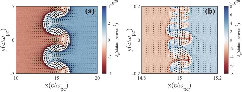
The formation of the out-of-plane current imbalance and the induced in-plane magnetic fields are presented in Fig. 1(a). The generation of the interfacial magnetic field can be described qualitatively as follows.²⁰ The shearing flows are charge- and current-neutral at the very beginning. The initial velocity perturbation δv_x transports electrons across the shear interface, instantly producing a current imbalance δJ_z due to the sharp transition in the shearing velocity field, as is shown in Fig. 1. The current imbalance then induces in-plane magnetic fields (δB_x, δB_y) on one side of the interface, which in turn enhances the velocity perturbation δv_x via the Lorentz force v₀ × δB_y. In the linear stage, the characteristic strength of the interfacial magnetic field structure is estimated as μ₀en₀v₀δv_xt.¹⁹ The enhanced velocity perturbation then leads to further electron transport across the velocity shear gradient in a feedback loop process, which acts as the basis for the MI growth in the linear stage.

The MI eventually enters a nonlinear stage when the growing magnetic fields become strong enough to significantly displace the electrons and distort the shear interface.²⁰ Such nonlinear distortion of the shear interface leads to the formation of electron surface current filament structures, which eventually induce a strong magnetic field structure extending around the entire interface, as can be seen in Fig. 1(a).

Considering a more universal physical picture, we remove the artificial perturbation of the velocity profile and set the initial temperature of the shear flows to 1 eV with a Maxwell–Boltzmann distribution so that the growth and saturation of thermally induced MI can be observed during the simulation time. The electron thermal velocity is slightly larger than the amplitude of the perturbation in the previous simulation. In this case, electron thermal expansion is expected to be the main mechanism responsible for electron transport across the interface and for formation of the current imbalance required to induce the dc magnetic field.

Magnetic field generation through thermal expansion is a similar physical process to the single-mode perturbation growth discussed in Subsection III A, which can be considered as a multimode development of the MI. Note that the direction of the interfacial magnetic field is not relevant to the modes of the perturbation, but depends only on the initial shearing settings, for which the possibility of multiple modes would not suppress the generation of the dc magnetic field from extending along one direction. However, the possibility of multiple modes suppresses the expansion of the mushroom-like structures, and thus limits the width of the interfacial magnetic field structure compared with the single-mode case with proper perturbation wave number k. In this situation, the early electron density protuberances generated from the thermal motion of electrons around the interface expand and start to interact magnetically with their neighborhoods. Small-scale current filaments are formed and subsequently merge into larger finger-like structures. The simulation results shown in Fig. 1(b) reveal excitation of the current filaments on either side of the shear interface and their merger into larger current structures as the instability grows. B_y is the dominant component of the interfacial magnetic field, while the averaged B_x and B_z components contribute little of the total field energy, namely, about 10⁻² and 10⁻³, respectively, at the moment presented in Fig. 1(b).

The growth of instability can be illustrated by the temporal evolution of the ratio between energy restored in the self-generated magnetic field and the total energy in the simulation box, as is shown in Fig. 2(a). The energy in the simulation box is strictly conserved, with a deviation less than 10⁻⁸. At the very beginning, the system is unmagnetized and current-neutral. The growth of instability is accompanied by an increase in the self-generated magnetic field. The magnetic field energy (and similarly the electric field energy) subsequently reaches a sufficiently large amplitude and saturates owing to the effect of magnetic trapping,²⁶ which makes it difficult to transport more electrons across the shear to form further current imbalance.³Figure 2(b) reveals that the growth rate of the MI increases with increasing initial plasma temperature and reaches a turning point where the induced electric and magnetic fields are comparable to the plasma thermal pressure. This conclusion is valid for a temperature range no higher than 3 keV for our simulation configurations. By contrast, in the ultra-hot regime (T_e > 50 keV), according to Alves et al.,²⁰ who took account of relativistic thermal effects and used an extension of the Jüttner distribution, an increase in the initial plasma temperature will cause a decrease in the MI growth rate. The great difference in parameter space (and thus in particle distribution) could lead to very different conclusions, and the transition between these two types of system is a topic that we are interested in for future study.

In another simulation, if a sinusoidal perturbation (like that in Sec. III A) is introduced into a warm shearing system with T_e = 0.1 keV, then growth of the seed perturbation will be accelerated owing to the existence of a thermally induced magnetic field that saturates much more rapidly. Interestingly, the mode of the added velocity perturbation will still determine the mode that eventually develops at later times. This coincides with what was found by Miller and Rogers,²⁷ who presented analytical results to show that the growth of MI is not sensitive to particle thermal dynamics in the MHD framework.

The thermally induced magnetic field in relativistic shear flows can extend all along the shear interface in our simulations and last long enough to cause a variety of electron and ion behaviors. To shorten the saturation time of the thermally induced magnetic field by a moderate amount and to better investigate the subsequent processes, we increase the initial plasma temperature to 0.1 keV while leaving the other parameters unchanged. The simulation results show that the generation of a strong interfacial field structure will first drive the electrons to move across the interface, forming a counterstreaming current sheet parallel to the initial interface. On the time scale of the electron response, the protons remain immobile, and thus an electrostatic field is formed by charge separation, as shown in Fig. 3(a). The electrostatic field and the Lorentz force (from the interfacial magnetic field) act as a restoring force on the electrons, which leads to the emergence of upper hybrid (UH) oscillation.²⁵ The dispersion relation for the electron oscillation in this scenario of unmagnetized, collisionless plasmas can be written asω2=ωce2+ωpe2+k2vth2,(1)where ω_ce = eB/m_ec is the electron cyclotron frequency in a magnetic field B, and v_th is the typical electron thermal velocity. In our specific simulation setup, it can be estimated that ω_pe ≃ 3.5 × 10¹⁴ rad/s and ω_ce ≃ 1.0 × 10¹⁴ rad/s, with a characteristic magnetic field strength of 6 × 10⁶ G, which leads to ΩUH=ωpe2+ωce2≃3.7×1014 rad/s. The sampling rate is then determined to be 2.6 × 10¹⁵ Hz based on the Nyquist–Shannon sampling theorem. The results of a frequency analysis of the electron density evolution of our PIC simulation are shown in Fig. 4 and are in general agreement with the theoretical analysis.

The characteristic strength of the dc magnetic field along the shear interface in plasmas of 0.1 keV saturated at 1.2 × 10⁷ G will be strong enough to affect proton dynamics within the simulation time, and thus ion mobility can no longer be neglected. Protons on both sides of the initial shear interface will be pushed apart by magnetic pressure, causing pileup of ions on either side of a gap. Note that we define the two borders of the separation gap as being where the averaged ion number density falls to one-half of the initial plasma density. We define the width between these borders as the separation width.

From Fig. 5(a), it can be seen that the separation process lags the development of the interfacial magnetic field in time, which can be explained by the fact that the separation can start to grow only when the interfacial magnetic pressure has become strong enough to overcome the ion thermal pressure. The simulation result shows that although the ions around the shear interface are slightly heated over time, their velocity distribution function deviates little from a drifting-Maxwellian distribution, and thus it is possible to obtain an ion “temperature” by statistical methods. By the time separation of ions begins to be observable, the effect of the ion thermal pressure gradient is negligible compared with that of the Lorentz force. Figure 6 illustrates two characteristic moments: one at which the magnetic field is dominant and the two shearing flows are expelled owing to magnetic pressure and the growth of the separation width is in the acceleration phase ^{[Fig. 6(a)]} and one at which the electric field has a greater impact on the ions, tending to prevent them from separating, and the growth of the separation width is in the deceleration phase ^{[Fig. 6(b)]}. Both of these moments and the corresponding separation states can be seen clearly in Fig. 5(a).

The separated ions will form a strong charge separation field and drag the trapped electrons from the region of strongest magnetic field, whereas the magnetic trapping will impede cross-interface transport of the electrons and thus saturate the magnetic field, which indicates that the broadening of the magnetic field structure and the separation of the ions have opposite effects on electron transport normal to the shear interface. The saturation of the interfacial magnetic field will be delayed if the mobility of the ions is taken into consideration.

The evolution of the ion separation process is caused mainly by the general effect of the interfacial magnetic field due to growth of instability, the electric field generated by charge separation, and the gradient in thermal pressure due to density pileup. From an MHD point of view, for one particular ionic fluid element on the boundary surface of the gap, the equation of motion can be written asminidvidt=nieE+vi×Bc−∇Pi,(2)∇⋅E=4πe(ni−ne),(3)B=Bsatey,(4)where B_sat is the saturated central magnetic field strength given by 1.3β0γ0(meωpec/e). Here, we adopt the β0γ0 scaling given by Grismayer et al.,¹⁹ and set the best-fit coefficient to 1.3 for 2D warm MI simulations with an initial shear velocity between 0.3c and 0.8c. It is reasonable to assume that the magnetic field is space- and time-independent in the equations above, since the separation happens on a space scale sufficiently small compared with the characteristic width of the dc magnetic field and on a time scale where the dc magnetic field has already reached saturation.

Another important assumption is made to further simplify the situation. The electrons are assumed to be fully trapped by the magnetic field. For a typical field strength of 10⁷ G in our 0.5c simulation, ω_ce/ω_pe = 0.58 and the electron Larmor radius is two orders of magnitude smaller than the electron inertial length c/ω_pe, which is also the characteristic length of the separation width in our simulations. As was shown in Sec. IV A, the high-frequency oscillation of the electrons inside the magnetic field structure means that it is reasonable to neglect the variation in electron density when considering ion-scale separation behavior.

By solving the equation of motion in x from a Lagrangian point of view, we can derive the equation that describes the separation behavior (adiabaticity and a linear density ramp are assumed):d2Wdt2=−γiTimiW−1−34ωpi2W+u0ωci,(5)where W is half of the separation width defined previously, γ_i = 3 is the one-dimensional adiabatic exponent, ωpi=4πn0e2/mi is the ion plasma frequency, and ω_ci = eB_sat/m_ic is the ion gyration frequency at B_sat. This equation is simplified when the ion thermal pressure term can be neglected, which is acceptable when the ion temperature remains below a few keV. Equation (5) can then be solved to giveW=43u0ωciωpi2+[ψ1⁡exp(iωpit)+ψ2⁡exp(−iωpit)],(6)where ψ₁ and ψ₂ are determined by the initial conditions. It can be seen that this solution consists of an equilibrium term and an oscillating term, the former of which is time-independent and can be used to examine the reliability of the model. In fact, it is more convenient to get the equilibrium term by simply setting the left-hand side of Eq. (5) to zero:Weq=23(u0ωci+u02ωci2−3(γiTi/mi)ωpi2)ωpi2.(7)This reduces to the first term on the right-hand side of Eq. (6) when the thermal pressure term is sufficiently small. Given the symmetry of the problem, the estimated separation width at equilibrium should beWeq≃83u0ωciωpi2=1.75×1013β02γ0n01/2(μm)(8)where n₀ is in m⁻³. The theoretical results at different initial shearing velocities are compared with the 2D PIC results in Fig. 7.

The theoretical results are slightly higher than the 2D PIC simulation ones, the main reason being the existence of a shear gradient layer (instead of the Heaviside function used earlier) between the two bulk plasmas on the ion time scale, which means the actual shear velocity of a fluid element is smaller than that in the initial situation. The formation of this shear gradient layer could be a combined effect of grad-B drift, E × B drift, and the noncontact frictional force due to electromagnetic instabilities.^25,28 Based on the simulation results, we can expect to obtain better agreement by altering the shear velocity to 0.95u₀, as can be seen in Fig. 7. The model breaks down in highly relativistic situations (β₀ > 0.8 in our initial configurations), where the theoretical prediction of the magnetic field strength we adopted no longer matches. The lower limit (∼0.2c) of the model is determined by competition between ESKHI and MI,¹⁹ since the latter is dominant only in relativistic regimes.

Alves et al.²⁰ have simulated the situation where the shearing flows are initially separated by a nanometer-scale vacuum gap and the situation with a smooth shear gradient of a certain length. In both situations, they have found that the growth rate of MI decreases with the gap/gradient length and that there is a critical length (in the vacuum gap situation) beyond which the growth of MI is largely restrained. Ion separation would have the same effect on the development of subsequent instabilities as in the density-gradient case. The critical gap length given in their theory is estimated as Lgmax≃2(γ02−1)γ0(c/ωpe), which is comparable to the equilibrium separation width W_eq, as can be seen in Table I.

2D3V PIC simulations have been performed at different time scales to investigate the evolution of the self-generated interfacial magnetic field of the MI and its impact on electron and ion dynamics. It has been found that the instability can be triggered by electron thermal motion and that its growth rate increases with rising initial plasma temperature, reaching a peak at an initial temperature of around 3 keV when the thermal pressure force is able to counteract the electric and magnetic forces that drive the unstable arrangement of the electron currents. In the case of a warm shearing configuration, the presence of the strong interfacial magnetic field will cause upper hybrid oscillation normal to the shear interface, as well as separation of ions on a longer time scale. A theoretical prediction of the equilibrium separation width has been presented and evaluated, and it has been found to match well with simulation results for initial shear velocities ranging from 0.2c to 0.8c. Scaling of the growth of such electron-scale instability and particle dynamics in experimental situations remains unexplored, and the coupling with other macroscopic (magneto)hydrodynamic instabilities is also a topic that we shall be investigating in the future.

References

[1] S. Chandrasekhar. Hydrodynamic and Hydromagnetic Stability(1961).