A variety of optical sensor technologies have been widely demanded and successfully adopted in modern electronic products from smartphones to autonomous driving systems. Optical Phased Array (Optical phased array, OPA) is one of the optical technologies that frequently comes under the spotlight lately for its potential use in autonomous vehicle and 3D sensing applications. OPA uses an array of optical antennas which can be individually addressed for phase (and sometimes amplitude) tuning in order to form a beam of light and to steer the beam to desired directions. Compared to radio frequency phased array that has been extensively used in many long distance ranging applications, optical phased array hasn't seen wide adoption partly due to the practical difficulty to pack a large number of individual optical antennas (and corresponding phase tuning elements) at distances comparable to optical wavelength. With the rise of integrated photonics, Si photonics in particular, people find ways to integrate many diffraction-limited optical elements close to each other at large scale by low-cost semiconductor wafer level process^[1-3]. Si photonics-based integrated OPA quickly becomes a hot topic in both academic research^[4-7] and entrepreneurial endeavors.

Integrated OPA is in its infancy for practical applications and many engineering challenges limiting its performance and practicality await for better solutions. One such challenge is to calibrate the almost random phase error (and to a lesser extend the amplitude error) among an array of waveguide-distributed antennas due to unavoidable processing errors (such as line edge roughness and lithography errors). Even very small width variations that modern semiconductor processes provide can cause large phase error and chaotic far-field patterns when such variations are accumulated throughout millimeter long waveguide routes which are required for even moderate number of antennas. Therefore, calibrating initial phase condition of an antenna array is required for every and each OPA product and the effectiveness and efficiency of the calibration is a key to successful commercialization.

Some mature calibration methods have used in radio frequency phased array. Such as near-field method^[8] requires measuring single antenna near-field data is not practical for OPA due to its micrometer size antenna. And the mutual coupling method^[9] requires a single antenna transmits signals and another antenna to receive. However the integrated OPA generally does not have single antenna transmission and reception function. Phase toggling method^[10] demands large and fine far field pattern measurement which makes corresponding optical calibration system complex and compute-intensive. None of these three calibration methods are suitable for integrated OPA.

Some generic optimization methods such as hill climbing, genetic algorithm, particle swam optimization, stochastic gradient descent algorithm and etc.^[11-14] can provide fairly good calibration in some cases. However all smart algorithms generally cannot avoid local extremum uncertainty (which is a severe issue for most OPA with larger-than-wavelength-spaced antennas) and are not scaled well with the size of the antenna array.

Rotating element Electric field Vector (REV) method^[15-16] is a more efficient far-field method while suffers possible π phase error when initial phases span the whole 2π space (which is common for optical band while less common in microwave band) at finite optical power measurement accuracy.

This paper propose a modified REV method that avoids the possible π phase error in traditional REV. The improvement in modified REV method has great implications in practical deployment of OPA products. This modified REV method is applied to a 9×9 OPA with unevenly spaced antenna array (for better side lobe suppression) and show that it produces statistically more accurate, predictable and converged calibration result.

Rotating element electric field vector method calculates the initial phases of each antenna by finding the maximum and minimum optical power at a fixed single far-field point while varying the phase of each antenna from 0 to 2π. For each antenna, from the measured phase shift ∆φ from the initial state to the maximum power state, the corresponding maximum power and the minimum power values, the phase shift from its initial state to the calibrated state (i.e. an ideal phase distribution for all antennas to maximize the power at the given far field point) of this antenna is calculated. Reset this antenna to its initial phase and repeat this process for the next antenna till the phase shift of all antennas is determined and the OPA is considered calibrated. The phase shift calculation in this method is correct in theory however in practice, as explained later, can produce π phase uncertainty error due to wide initial error range (0~2π) and finite optical power measurement accuracy.

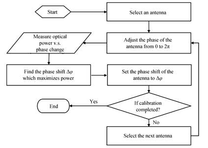
Instead, modified REV method lets ∆φ as the phase shift from the initial state to the calibrated state and set the antenna to this maximum power phase when repeating the same calibration step on the next antenna. This process quickly converges and approaches to the ideal calibration condition with the number of calibrated antennas. And this simple approach avoids π phase uncertainty and do not rely on precise maximum and minimum power measurement data. The calibration process is shown in Fig.1 and the theory is explained in details below.

The electric field of the nth antenna at a fixed far-field point Q is

where α, β and r is the coordinates of point Q in polar coordinate system, A_n (α, β, r) is the amplitude of the antenna, ω is the optical frequency, r_n is the distance vector from the antenna to the point Q, φ_n is the initial phase of the antenna, and e is unit vector determined by polarization.

In practice the interested far field target is significantly farther in distance than the size of the OPA thus the directions of electric field and distance vectors of all antennas can be approximately considered the same. In addition, as all antennas share a single coherent light source the polarization of every antenna is the same. Eq. (1) can then be simplified to scalar form. The total electric field at point Q is

where ${\phi _n} = {\varphi _n} - k{r_n}$ is the phase of the nth antenna at point Q. The intensity is

When the phase of the mth antenna is changed by ∆φ, the intensity becomes

Define

where E$ _{ - m}$ represents the sum of the electric fields of all antennas except the mth, A$ _{ - m}$ is the amplitude of E$ _{ - m}$, and v_m and w_m are the real and imaginary part of the E$ _{ - m}$, respectively.

The intensity I(∆φ)can then be expressed as

A derivative calculation shows the following condition must be met at an extremum of I(∆φ)

The intensity at Q reaches its maximum when $\Delta \varphi + {\phi _m} = {\rm{ }}{\rm{arctan }}({w_m}/{v_m}) $as shown by the second derivative of I(∆φ) without losing generality by assuming A$_m $ > 0

and the maximum intensity I_max is

It simply implies that the intensity of point Q reaches its maximum with the mth antenna and the combined field of the rest of the antennas are in-phase. This simple principle guides the whole calibration process. After the ∆φ of each antenna is obtained by varying its phase till maximum measured optical power at Q, the antenna is fixed at this phase and the next antenna is calibrated to the next maximum intensity condition. Repeat this process until all antennas are calibrated and set to their maximum intensity phase. The principle also guarantees the monotonic increase of the measurement optical power which helps reduce any possible ambiguity during the process. This method can be used for calibrating an OPA antenna array distributed in any patterns and does not demand any particular order in selecting antennas.

The whole process may be explained more intuitively in Fig.2(a)~(f). The related electrical field is drawn in a vector plane where the length and the angle from x-axis of a field represent its absolute amplitude and phase respectively. The following text refer to a field vector in this representation as opposed to a real space representation.

In practice when measurement error inevitably present, the final antenna array phase condition as well as the maximum intensity at Q may still be slightly off from their ideal values, even so, the following analysis shows the calibration well approaches the ideal condition, traditional REV also presents similarly if not worse results. In practice, the calibration process in production demands a statistically predictable and converged result.

For practical considerations, the errors need be analyzed in this method. It can be seen that the calibrated field vectors of the mth and the (m+1)th antennas that are aligned to E$- m$ and E_-(m+1), respectively, as shown in Fig.2(e) are generally not aligned with each other. Therefore at least one of the calibrated phase values of mth and (m+1)th antennas differs from its ideal value and it represents an intrinsic error of the method. However, as explained, such error does not pose significant overall calibration error and the error is more limited or converged than that in traditional REV method when measurement errors exist.

As shown in Fig.2(f), the relative intrinsic phase error of a certain antenna (m+1) reaches its maximum in this case and the error, the phase difference between the (m+1)th and the mth antenna, in general satisfies

where A_(m+1) is the amplitude of the (m+1)th antenna; $ E_0 $ is the combined electric field at point Q before calibrating the (m+1)th antenna. It implies δφ_(m+1) continues to decrease with the increase of the number of the calibrated antennas as |E₀| becomes larger when more antenna field vectors getting approximately aligned.

For example, after the first antenna is calibrated, $ |{E_0}| \ge {A_1} \cong {A_2}$, the phase difference between the second and the first antenna

while for the third antenna to the calibrated, $|{E_0}| \ge \sqrt 2 {\rm{ }}{A_3} $, the phase difference

and it can be easily seen that δφ continues to reduce as more antennas are calibrated.

In an OPA where the phase error is mostly introduced by waveguide size variations, antennas initial phases tend to be widely distributed thus the intrinsic phase error after calibration also randomly distributes within ±δφ and the calibration imperfection caused by such distributed error is generally far less severe than the worst case scenario. In addition, if higher calibration accuracy is required, the same process can be repeated. And since |E₀| becomes significantly larger after the first calibration process the intrinsic error becomes even smaller. Furthermore it is generally sufficient to only perform the second calibration on first few antennas whose phase errors are relatively larger than others.

Another type of error rises from errors in measurement (mainly measured optical power) and in calculations using the measurement data (phase change between initial to maximum power conditions). In traditional REV, such measurement error becomes more severe due to the way of calculating phase values that can introduce possible π phase error. The equation to calculate the initial phase of an antenna in traditional REV method is

where ∆φ_pmax is the phase shift from the initial state to the maximum power state; p_max and p_min are the maximum and minimum power at point Q, respectively.

The arctan function produces a value between [-π/2, π/2] while the possible true phase difference ranges a whole 2π. It requires the algorithm to decide whether or not to purposely add a π to its solution based on the value of ∆φ_pmax. Such decision in principle has no problem, however, it presents possible error when the phase change from its initial value to the measured maximum power point occurs close to ±π/2 at which small optical power error may produce completely wrong determination.

As shown in the second section, even a 0.1% intensity error can cause poor calibration results. In a microwave radar, where the initial phase shifts of antennas are generally not as widely diverged as in an OPA, such issue is not as severe. Such practically inevitable error is considered in the second section and its effect between traditional REV and modified REV methods is compared.

To test modified REV calibration method, the following simulation work is performed with a 9×9 two-dimensional optical phased array operating at 1 550 nm wavelength. Assuming all antennas share the same emission profile including intensity and far-field distribution, the optical power non-uniformity introduced by some Si photonics integrated OPA designs (e.g. power splitting^[17-18] or cascaded power tapping^[19-20]) has tolerable detrimental effect.

To simulate a real-world process of finding the maximum optical power at Q and calculating the phase shift, the phase can only be varied in a finite step provided by the resolution of a digit-to-analog converter (Digit-to-Analog Converter, DAC). Considering a DAC resolution ranges from 3-bit to 8-bit (for 0~2π range), its effect is tested on calibration result.

A small Gaussian-distributed error is introduced to the far field optical power measurement data. In practice, this error rises from multiple sources including IR camera measurement inaccuracy, side lobe light scattered by a test system, scattered light from chip-coupled light source, stray ambient light, etc. The Gaussian error is within ±0.1% (at 3σ) of the peak far field intensity. However it has a non-negligible effect on calibration result.

First, the far field of the OPA is calculated with ideal initial phase condition, i.e. phases are equal for all antennas as shown in Fig.3(b) and the result is shown in Fig.3(a). The far field are the intensity values at the spherical surface originated from the OPA (x=0, y=0) with a radius of 1 m and (φ, θ) represent the angles from z-axis in x-z and y-z planes respectively. A special case with intensity vs. θ at φ=0 shows one of the directions with the worst side lobe suppression which generally limits this OPA system to about 60⁰ Field of View (FOV). A typical far-field, antennas phase map, and far-field intensity with θ at φ=0 with randomly distributed initial phase between 0 and 2π are shown Fig.3(d)~(f) respectively. The far field intensity is scaled with the same range as in the ideal case. It can be easily seen that a widely distributed initial phase errors generally destroy constructive interference and result in chaotic far field and much lower peak values. The same three plots after the initial phase errors are calibrated by modified REV method are shown in Fig.3 (g)~(i). The calibration is processed in one pass with 8-bit phase tuning resolution and Gaussian intensity error as mentioned earlier. It can be seen that the calibrated results agree very well with the ideal phase condition results and the system is considered to be calibrated (although the initial phases at some antennas may be off from their ideal values).

The 1D far field in Fig.3 (c) may be easily use as a visual benchmark to compare calibration results among cases while it is more convenient to use the relative intensity, i.e. scaled with the same range as the ideal case, at Q (θ=0, φ=0) as a figure-of-merit to quantitatively compare the statistical calibration performance by different methods at different conditions. It is also called as calibrated intensity in following texts.

To compare the calibration performance between modified REV (mREV) and traditional REV as well as to test the effect on phase tuning resolution, calibration process is performed by both mREV and REV for 1 000 cases of randomly generated (within 0~2π) initial phase maps with phase tuning resolutions ranging from 3-bit to 8-bit. The results are summarized in Fig.4 (a). It can be seen that at any phase tuning resolution the overall calibration performance of mREV is much better than REV in terms of the average calibrated intensity and its error (i.e. root-mean-square error). To show how the calibrated intensity statistically distributes, the 6-bit phase resolution case is picked and plot the probability distribution of calibrated intensity of the 1 000 cases processed by mREV and REV, respectively, in Fig.4(b). It clearly shows that the calibrated intensity of REV is less accurate and more diverged than that of mREV. In practice, it's obviously preferred to have a robust product calibration process with results produced by mREV.

For mREV, the increase of average calibrated intensity with phase tuning resolution, i.e. number of bits, is easy to understand as the accuracy of ∆φ for each antenna increases. The same analysis doesn't apply to the REV cases as shown in Fig.4 (a) where the average calibrated intensity is slightly higher at lower resolution while the maximally achieved calibrated intensity (upper boundary) presents at medium resolutions. As already known for REV, another source of error, π phase error in certain initial phase conditions, sometimes determines overall calibration performance. At low resolution, i.e. smaller bits, although the phase accuracy is low, the chance to make a π error is also low as the intensity difference between two adjacent phase tuning steps is often too large to produce incorrect determination even with the presence of power measurement errors.

The above analysis explains the histograms of the calibrated antennas phases. Some typical histograms are shown in Fig.5. The calibrated phases are generally more concentrated within a narrow range in mREV cases. While in cases calibrated by traditional REV, although phases of many antennas are also within a similar narrow range there are always certain phases located in another π-shifted range and such errors cause poor calibration result.

For experimentally validating the simulation results, a 9×9 two-dimensional optical phased array device is calibrated, as shown in Fig.6(a). The OPA device is designed as a non-uniform antenna array and fabricated with silicon photonics technology. This device has 81 thermal phase shifters and each of them is independently adjustable. A 1 310 nm laser is coupled into the OPA chip through a polarization controller and a grating coupler. A computer, adjustable DC voltage-stabilized power supply and 81-channel digital-to-analog converter are used to control the voltage applied to each antenna unit. Applying a series different voltages on a phase shifter, the phase of the optical emission from the antenna unit is tuned from 0 to 2π. Then, a series different far field images are collected by a high numerical aperture (NA=0.5) lens and captured with InGaAs infrared camera (256×320 pixels), as shown in Fig.6(b).

Using mREV method to calibrate the device, computer program automatically searches what voltage make the far field pattern closest to the target pattern, then applies the voltage on the phase shifter. Repeating this process on all phase shifters, the calibration experiment is finished. The whole calibration process is easy to operate, just input the voltage sweep range, step length and sequence of phase shifters, the program will complete the calibration.

The initial grating lobe suppression ratio of this OPA device is 2.12 dB, as shown in Fig.7 (a)~(c). After calibration with mREV method, the grating lobe suppression ratio achieves 4.68 dB, as shown in Fig.7 (d)~(f). Comparing with the initial far-field pattern, in the calibrated pattern more energy is concentrated on the main lobe, meanwhile the grating lobe is weakened a lot. Although the grating lobe suppression ratio doesn't reach the design value (6 dB), it is not because of the mREV method but because of on-chip thermal crosstalk and manufacturing errors.

The paper presents a modified rotating element electric field vector method for calibrating the antenna array initial condition of an optical phased array with arbitrary initial phase distribution, the number of antennas and the arrangement of the antennas. The numerical simulation results show that the method can calibrate ideal far-field intensity distribution to practically sufficient accuracy. Even with the presence of significant random measurement errors representing realistic situations in practice, the main lobe intensity can statistically reach more than 90% of the ideal case. In addition, the results show a much less scattered error range, which is essential for calibration in practical deployment, compared to the results by traditional REV at the same simulated realistic conditions. The improvement in both accuracy and precision of the initial phase condition calibration by the modified REV results from the absence of π-shift ambiguity which is inevitable, but less severe in radio frequency phased array applications, in the traditional REV method.Due to the improved accuracy, precision and stability, the presented modified REV method provides great benefits in practice when calibrating OPA products with large number of antennae and phase shifters such as those are made by integrated photonics. The complexity in calibration and testing is currently one of the obstacles to accelerate the deployment and mass production of OPA devices, and the modified REV method can help make the progress.The experiment proves part of the simulation results, in future, more OPA devices should be calibrated to prove all of the simulation results.

References

[4] RAVAL M, POULTON C V, WATTS M. Unidirectional waveguide grating antennas f nanophotonic phased arrays[C]. Conference on Lasers ElectroOptics, 2017: STh1M.5.
[19] HASHEMI H. Largescale monolithic optical phased arrays[C]. Optical Fiber Communication Conference, 2019: Tu3E.5.
Set citation alerts for the article
Please enter your email address
© Copyright 2018-2021 | Chinese Laser Press. All Rights Reserved 沪ICP备15018463号-20