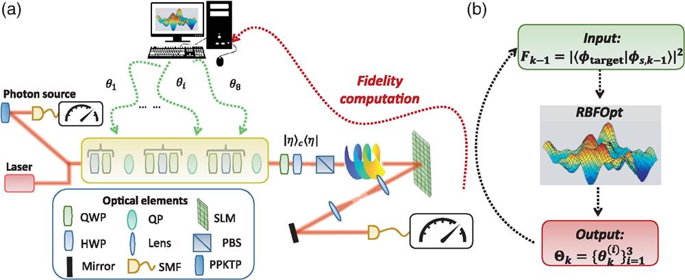
Fig. 1. Experimental apparatus. (a) The engineering protocol has been tested experimentally in a three-step discrete-time QW encoded in the OAM of light with both single-photon inputs and classical continuous wave laser light (CNI laser PSU-III-FDA) with a wavelength of 808 nm. The single-photon states are generated through a type-II spontaneous parametric down-conversion process in a periodically poled KTP crystal. The input state is characterized by a horizontal polarization and OAM eigenvalue m=0. Each step of the QW is made by a coin operator, implemented through a set of waveplates (QWP–HWP–QWP), and the shift operator, realized by a QP. To obtain the desired state in the OAM space, a suitable projection in the polarization space is performed through a quarter-waveplate, a half-waveplate, and a polarizing beam-splitter. The measurement station of the OAM-state is composed by an SLM followed by a single-mode fiber, and the coupled signal is measured through a power meter, in the classical regime, or an avalanche-photodiode detector, in the quantum one. In particular, in quantum optimizations, pairs of photons are generated, and heralded detection is performed, computing the two-fold coincidences between the detectors clicks from the QW evolved photon and the trigger one. The RBFOpt ignores the features of the experimental implementation that is seen as a black box. The algorithm has access only to the Θ parameters of the coin operators and to the computed fidelity. (b) During the iterations of the algorithm, the RBFOpt samples the black-box function to construct a surrogate model that is employed in the optimization. In the k’th iteration, the algorithm receives as input the fidelity computed in the previous iteration and uses it to improve the surrogate modeling. Moreover, the new parameters Θk are computed based on the optimization process. This procedure is repeated for each iteration of the algorithm.

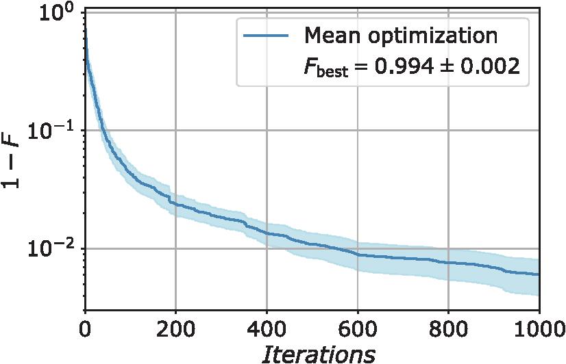
Fig. 2. Simulated optimization: infidelity 1−F obtained at different stages of the optimization. We test the algorithm on 10 random target states, repeating the optimization 10 times for each. The reported results are obtained as the mean over the average behavior for each of the 10 states. The highest average fidelity obtained is 0.994±0.002. The shaded area represents the standard deviation of the mean.

Fig. 3. Experimental results: (a) minimization of the quantity 1−F averaged over the algorithm performances for different experimental states. The mean maximum value reached is 0.983±0.004. (b) Ratio between the maximum experimental values of the fidelities resulted after the optimization F(Θopt) and the fidelities measured with the theoretical parameters F(ΘTh). For each engineered state, the ratio is higher or compatible with the value 1 highlighted by the dashed line. This confirms that the adopted algorithm can reach performances compatible or even superior with respect to the one obtained with the direct method presented in Ref. 24 that considers ideal experimental platforms. In this sense, the algorithm can take into account and compensate for the experimental imperfections. All of the error bars reported are due to laser fluctuations affecting each measurement and are estimated through a Monte Carlo approach. (c) Comparison between the performances reached in 100 iterations using classical or single-photon input states. In yellow is reported the area between the best and worst optimization performed in the classical case. The blue and violet curves are associated with the minimization of the quantity 1−F averaged over five different optimizations for the state SR1−1 engineered in the quantum domain. In particular, the raw data are shown in violet, whereas the data after accidental counts subtraction are in blue.

Fig. 4. Experimental perturbation results. (a) Optimization under external perturbation of the quantity 1−F for the state |1⟩. The iterations in which a perturbation δ occurs are highlighted by a vertical red line (second step HWP) or by a vertical green line (third step QWP), and a vertical orange line highlights the iteration in which the algorithm is restarted. (b) Mean ratio between the best value obtained for the fidelity after (Fbesta) and before (Fbestb) the perturbation for the different engineered states. The ratio is close to or higher than 1 for all of them, which showcases that the algorithm is able to reobtain and eventually improve the best value sampled before the perturbation. All of the error bars reported are due to laser fluctuations affecting each measurement and are estimated through a Monte Carlo approach.

Fig. 5. Scalability: the plot shows the mean number of RBFOpt algorithm iterations as a function of the black-box problem parameters. Here, the optimization process is interrupted when a value of the fidelity between the target state and the one proposed by the algorithm of at least 98% is reached. For each configuration, the iteration values are obtained by averaging more than 50 random target states and simulating experimental noise using binomial and Poissonian distributions. The uncertainty associated with each point is provided by the standard deviation of the mean.

Fig. 6. Comparison between different optimization algorithms: the plot reports the simulated performances of three different algorithms averaged over the optimization of 10 different states, each of which is repeated 10 times. Dotted blue, dashed green, and continuous orange lines report the trends corresponding to Powell, random search, and RBFOpt, respectively. RBFOpt is found to perform significantly better than the alternatives in most cases. All curves are generated simulating experimental noise with both Poissonian () and binomial fluctuations.

Table 1. The parameters used in the study of the optimization under perturbations for the engineered states. In the second column, we report the values of the perturbation occurrence probability q, whereas in the third column, we report the threshold values t used for deciding the algorithm restart.

Table 2. The RBFs exploited by the RBF algorithm and the degree of the polynomial used in the construction of the surrogate model.^70,71,84,85 When d=−1, the polynomial is removed from Eq. (3).