Semi-supervised semantic segmentation based on Generative Adversarial Networks for remote sensing images

Yu-Xi LIU; Bo ZHANG; Bin WANG

doi:10.11972/j.issn.1001-9014.2020.04.012

Journals >Journal of Infrared and Millimeter Waves >Volume 39 >Issue 4 >Page 473 > Article

Journal of Infrared and Millimeter Waves
Vol. 39, Issue 4, 473 (2020)

Semi-supervised semantic segmentation based on Generative Adversarial Networks for remote sensing images

Yu-Xi LIU, Bo ZHANG, and Bin WANG^*

Author Affiliations

Key Laboratory for Information Science of Electromagnetic Waves (MoE), Fudan University, Shanghai200433, China

show less

DOI: 10.11972/j.issn.1001-9014.2020.04.012 Cite this Article

Yu-Xi LIU, Bo ZHANG, Bin WANG. Semi-supervised semantic segmentation based on Generative Adversarial Networks for remote sensing images[J]. Journal of Infrared and Millimeter Waves, 2020, 39(4): 473 Copy Citation Text

show less

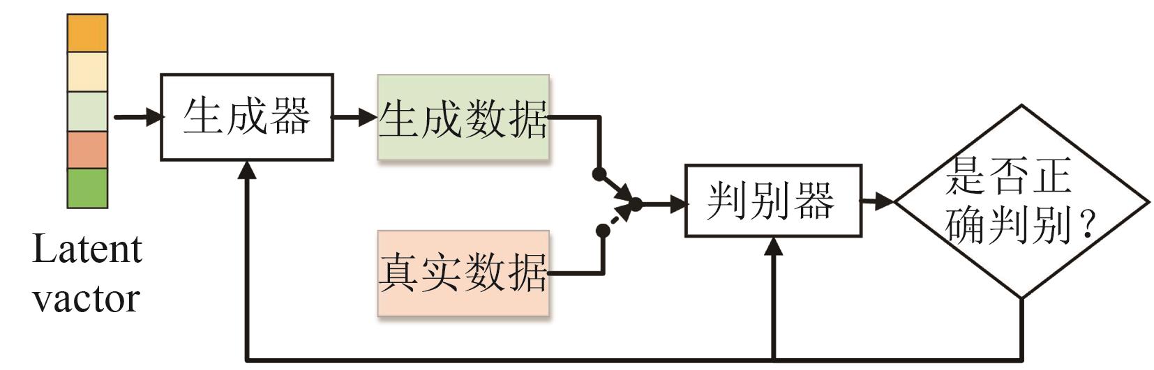
Fig. 1. The framework of Generative Adversarial Networks

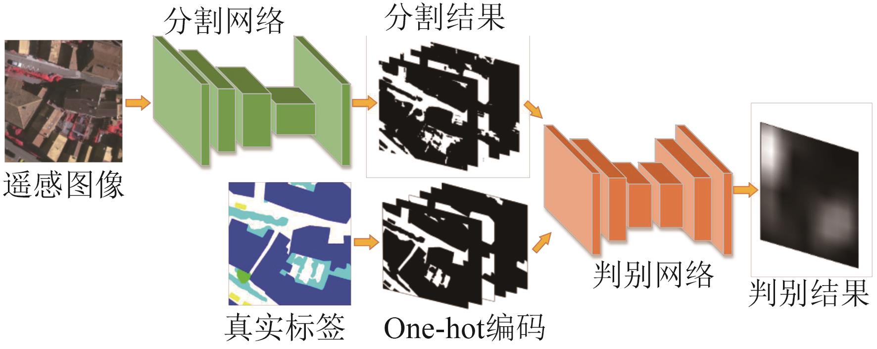
Download full size | View in the Article

Fig. 2. The overall framework of the proposed method

Download full size | View in the Article

Fig. 3. Illustration of the ISPRS 2D Vaihingen Labeling dataset (a) the entire remote sensing image, including near-infrared, red and green bands, (b) partial remote sensing image numbered 2, and (c) corresponding label map and its legend

Download full size | View in the Article

Fig. 4. Illustration of cropping the entire image

Download full size | View in the Article

Fig. 5. Illustration of confusion matrix

Download full size | View in the Article

Fig. 6. Visual comparison of segmentation results among the proposed method and other state-of-the-art models on test set: (a) image for segmentation, (b) ground truth label map, (c) UPB, (d) ETH_C, (e) CAS_Y3, (f) ITC_B2 (g) VNU4, (h) CASZX1, (i) UFMG_3, and (j) the proposed method

Download full size | View in the Article

类型	比例	Method	Imp Surf	Building	Low_veg	Tree	Car	OA	Mean F1
有监督	1	Baseline	86.3	92.6	70.7	85.6	69.9	85.3	81.0
		$+ L_{a d v}$	88.8	93.9	75.6	87.9	77.6	87.7	84.7
		$+ L_{a d v_a t t}$	89.0	94.1	75.6	88.0	78.4	88.0	85.0
半监督	1/4	Baseline	83.0	90.7	62.7	83.7	62.0	82.0	76.4
		$+ L_{a d v}$	86.9	93.2	71.7	86.8	74.9	86.2	82.7
		$+ L_{a d v_a t t}$	87.8	93.8	73.2	87.3	75.0	86.8	83.4
		$+ L_{a d v_a t t} + L_{s e m i}$	87.8	93.9	73.8	87.4	76.2	87.2	83.8
	1/8	Baseline	80.0	87.9	60.1	81.0	49.1	79.1	71.8
		$+ L_{a d v}$	85.5	91.3	70.2	86.0	69.3	84.5	80.5
		$+ L_{a d v_a t t}$	86.4	92.1	71.6	86.6	72.9	85.5	81.9
		$+ L_{a d v_a t t} + L_{s e m i}$	86.7	92.1	74.2	87.0	73.1	86.1	82.6

Table 1. 不同标签样本比例下各部分提升效果比较

View in the Article

比例	Method	Imp Surf	Building	Low_veg	Tree	Car	OA	Mean F1
1/4	Baseline	83.0	90.7	62.7	83.7	62.0	82.0	76.4
	SSGAN^[19]	83.6	91.0	63.9	84.1	65.7	82.9	77.7
	Semi-SegGAN^[17]	87.3	93.3	73.5	87.1	75.7	86.5	83.4
	本文方法	87.8	93.9	73.8	87.4	76.2	87.2	83.8
1/8	Baseline	80.0	87.9	60.1	81.0	49.1	79.1	71.8
	SSGAN^[19]	81.1	88.3	62.5	82.0	54.3	81.6	73.6
	Semi-SegGAN^[17]	85.9	91.5	70.8	86.1	72.3	84.9	81.3
	本文方法	86.7	92.1	74.2	87.0	73.1	86.1	82.6

Table 2. 与其它半监督语义分割方法在验证集上的结果对比

View in the Article

λ_adv	λ_semi	T_semi	OA	Mean F1
0.01	0	N/A	85.5	81.9
0.01	0.01	0.2	85.6	82.0
0.01	0.1	0.2	86.1	82.6
0.01	0.2	0.2	85.8	82.3
0.01	0.1	0.1	85.7	82.1
0.01	0.1	0.2	86.1	82.6
0.01	0.1	0.3	85.9	82.4
0.001	0.1	0.2	85.4	81.8
0.01	0.1	0.2	86.1	82.6
0.1	0.1	0.2	84.9	80.9

Table 3. 超参数、和取值分析

View in the Article

$γ$	OA	Mean F1
0	85.1	81.6
0.5	85.3	81.8
1	86.1	82.6
2	85.5	82.0
5	85.5	81.8

Table 4. 超参数取值分析

View in the Article

Method	Imp Surf	Building	Low_veg	Tree	Car	OA	Mean F1
UPB^[9]	87.5	89.3	77.3	85.8	77.1	85.1	83.4
ETH_C^[25]	87.2	92.0	77.5	87.1	54.4	85.9	79.6
CAS_Y3^[6]	89.6	91.5	82.0	88.3	68.4	87.8	84.0
ITC_B2^[7]	90.1	93.5	82.1	88.3	77.1	88.4	86.2
VNU4^[26]	91.2	93.6	81.5	88.5	77.7	89.0	86.5
CASZX1^[27]	91.3	93.9	81.9	88.3	77.6	89.0	86.6
UFMG_3^[28]	90.7	94.3	82.5	88.5	77.4	89.0	86.7
所提议方法	92.7	95.1	84.3	89.4	86.2	90.6	89.5

Table 5. 与其它性能优异方法的测试集结果对比

Yu-Xi LIU, Bo ZHANG, Bin WANG. Semi-supervised semantic segmentation based on Generative Adversarial Networks for remote sensing images[J]. Journal of Infrared and Millimeter Waves, 2020, 39(4): 473

Download Citation

Tools

Save the article for my favorites

Paper Information