- Spectroscopy and Spectral Analysis
- Vol. 42, Issue 11, 3559 (2022)
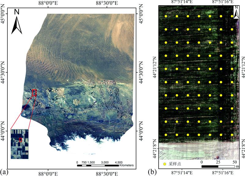
Fig. 1. The study area and distribution of sampling points
(a): RGB true color image of Fukang city and study area using Gaofen-1; (b): Sampling points
(a): RGB true color image of Fukang city and study area using Gaofen-1; (b): Sampling points
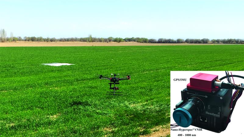
Fig. 2. UAV operation and UAV-based hyperspectral sensor
Fig. 3. Descriptive chart of the sample sets
Fig. 4. Hyperspectral images after FOD processing
(a): Hyperspectral image cube; (b)—(u): Processing results of 0.1 to 2 orders
(a): Hyperspectral image cube; (b)—(u): Processing results of 0.1 to 2 orders
Fig. 5. Spectral preprocessed by different FOD
Fig. 6. The correlation coefficient between band and SMC under different FOD pretreatments
(a): Heatmap; (b): Maximum correlation coefficient
(a): Heatmap; (b): Maximum correlation coefficient
Fig. 7. Scatter plot of measured SMC and estimated SMC
Fig. 8. SMC spatial distribution under the optimal model
Fig. 9. Bands importance under different FOD pretreatment
|
Table 1. Comparisons of GBRT models based on different modeling strategies

Download Citation

Set citation alerts for the article
Please enter your email address
© Copyright 2018-2021 | Chinese Laser Press. All Rights Reserved 沪ICP备15018463号-20